Math 344: Calculus III

14.1 Functions of Several Variables

---

14.1.1 Functions of Two Variables

Definition

A function $f$ of two variables is a relation that assigns to each ordered pair $(x,y)$ in a set $D$, a subset of the plane, $D\in\mathbb{R}^2$ a unique real number denoted $f(x,y)$. The set $D\in\mathbb{R}^2$ is called the domain of the function. Likewise the codomain of the function is a subset $E$ of the real numbers such that $f(x,y)\in E$ for every ordered pair $(x,y)\in D$. The codomain of such a function is often taken to be the entire real line. We write

$$ f:D\rightarrow\mathbb{R} $$
Like functions of one real variable, a function $f$ must produce a unique value $z\in E$ for every ordered pair $(x,y)\in D$. Output $z = f(x,y)$ is called the image of ordered pair $(x,y)$.

However this is not true for the codomain. Often the codomain is a larger set than the set of all images of elements of the domain. The set of images in the codomain

$$ \left\{ z = f(x,y)\,:\,(x,y)\in D\right\} $$
is called the image of function $f$.

The variables that represent the ordered pairs are called independent variables , and the variable that represents the output is called the dependent variable .

We can visualize a function of two real variables as a surface in three dimensional space. Every point in the image of our function corresponds to an ordered triple

$$ \langle\, x,y,z\,\rangle \longleftrightarrow \langle\, x, y, f(x,y)\, \rangle $$
Since we have exactly one value $z$ for every point on the $xy$-plane, the graph of a function of two real variables; that is the locus of all points $\langle\, x,y,f(x,y)\, \rangle$, is a surface in three dimensional space.

14.1.2 Equation Defined Functions of Two Variables

Example 14.1.1

Define function $f:\mathbb{R}^2\rightarrow\mathbb{R}$ by the equation
$$ z = x^2 + y^2 $$

• By this we mean that the domain of our function is the entire plane $(x,y)\in(-\infty,\infty)\times(-\infty,\infty)=\mathbb{R}^2$
  
  

• The range of our function is the real line $(-\infty,\infty)=\mathbb{R}$.
  
  

• The image of our function is the set of real numbers $R = \left\{z\in\mathbb{R}\,:\,z=x^2+y^2\right\}$
  
  

The graph of $f(x,y) = x^2 + y^2$
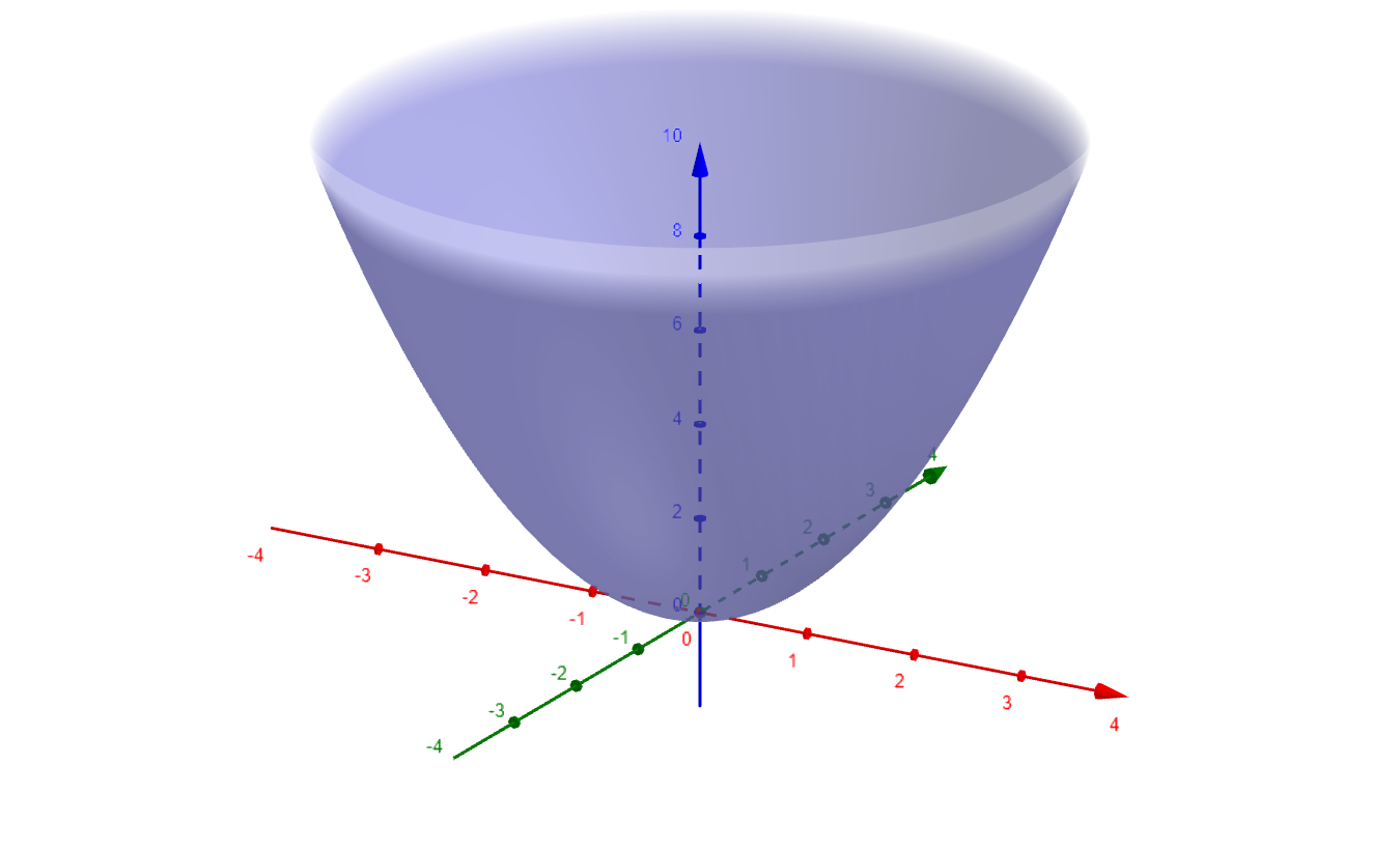
Figure 1

As every output $z$ is a sum of two nonnegative real numbers $x^2+y^2$, the image of $f$ is the interval $R = [0,\infty)$.

Example 14.1.2

Just as in previous calculus courses one often encounters an equation. The reader must infer the largest possible domain and codomain from the equation. Suppose we have the equation

$$ f(x,y) = \dfrac{\sqrt{x + y + 1}}{x - 1} $$

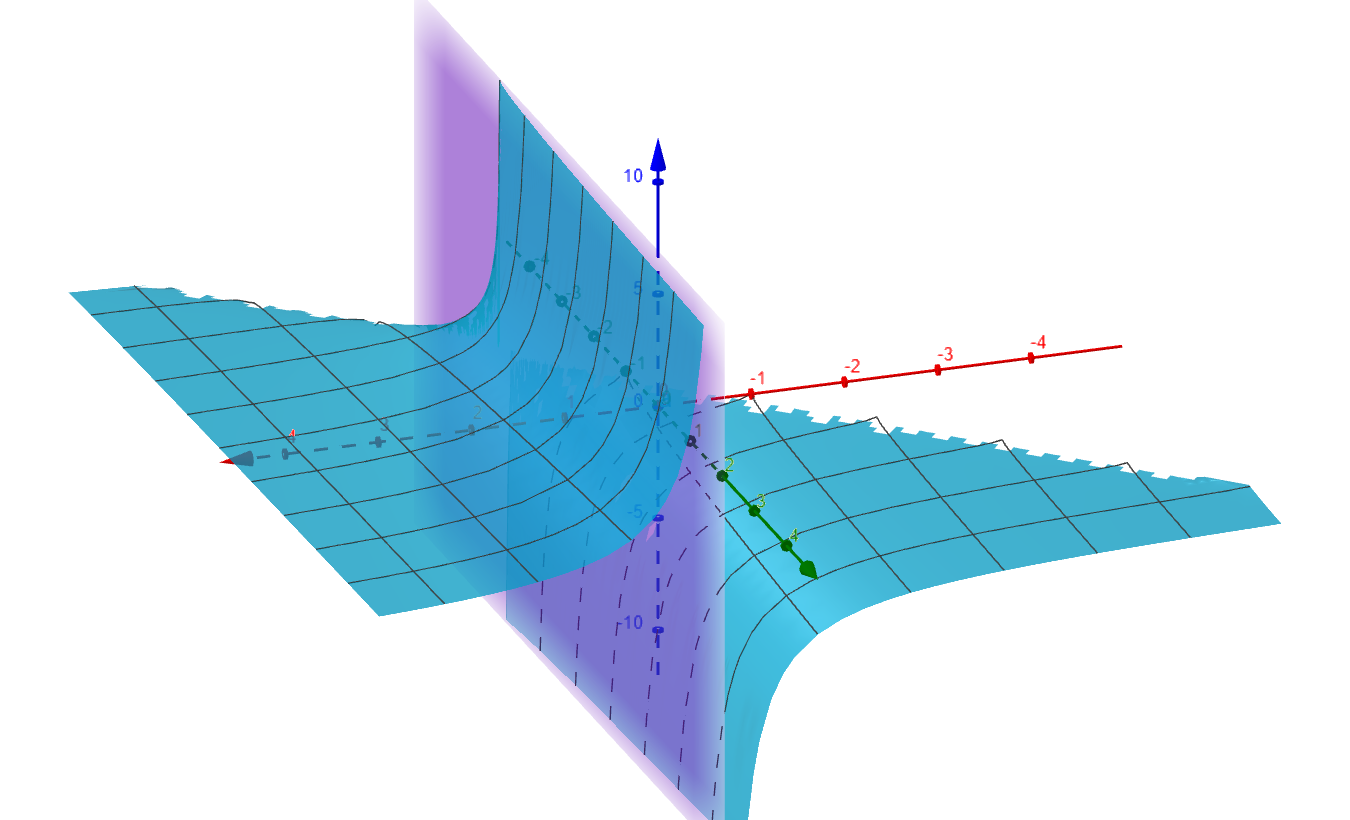
Figure 2

Notice that the surface is asymptotic to the plane $x=1$. The domain must satisfy the equation

$$ x + y + 1 \ge 0 $$
since sqrt is not defined for negative values if we want a real result. We can simplify this equation

$$ y \ge -x - 1 $$
Furthermore we have the $x\neq 1$ otherwise we will have zero in the denominator of the expression for $f(x,y)$. That is this function $f(x,y)$ is not defined for any values for which $y \lt -x - 1$, nor defined if $x=1$. We can graph the domain

$$ D = \left\{ (x,y)\,:\, y\gt-x-1,\ x\neq 1\right\} $$

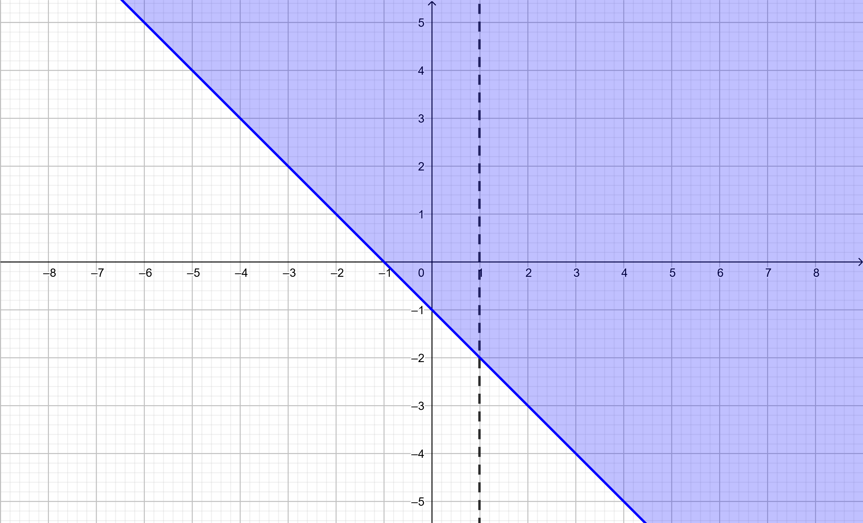
Figure 3

We can graph the domain in the $xy$-plane and the surface in the same plot

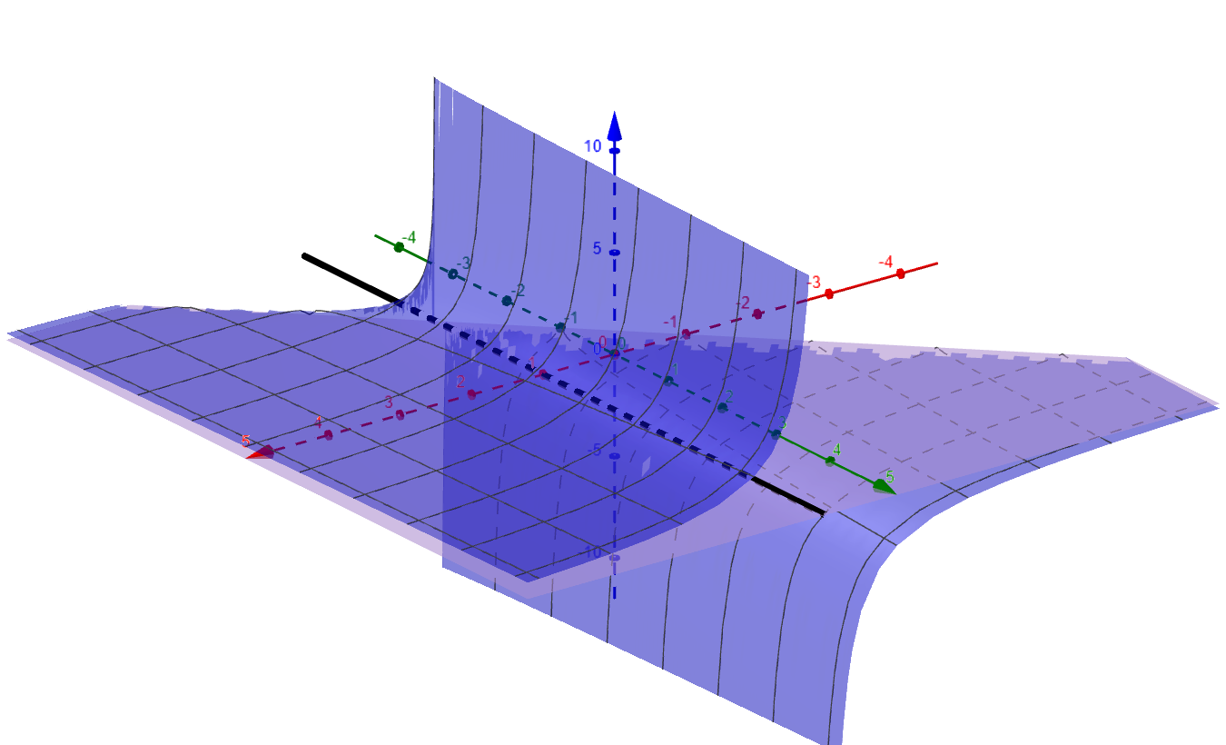
Figure 4

Using the graph, the image of this function excludes the real value zero since the numerator $\sqrt(x+y+1)\ge 1$ for all $(x,y)\in D$. Hence the image of $f$ is $(-\infty,0)\cup(0,\infty)$. The minus sign for sets is the backslash so we may denote the image

$$ R = \left\{ \dfrac{\sqrt{x+y+1}}{x-1}\,:\,(x,y)\in D\right\} = (-\infty,0)\cup(0\infty)=\mathbb{R}\setminus 0 $$

14.1.3 A Table Defined Function of Two Variables

The heat index is often used to describe the apparent severity of the heat. This index $H$ is a subjective measure of how hot one feels . Heat index is a function of relative humidity and air temperature. The values in this table indicate heat index in shady regions. Exposure to full sunlight can increase heat index by as much as $15^{\circ}$F. Exposure to hot dry winds can increase the heat index to very dangerous levels.

Example 14.1.3

Relative Humidity (%)

T \ %	16	20	24	28	32	36	40	44	48	52	56	60	64	68	72	76	80	84	88	92	96	100	% / T
124	130	138	146	155	165	175																	128
120	124	130	137	144	152	161	170	180															120
116	117	122	128	134	140	148	155	164	172	182													116
112	112	115	120	124	130	136	142	149	156	164	172	181											112
108	106	109	112	116	120	125	130	135	141	148	155	162	170	178									108
104	101	103	105	108	111	115	119	123	128	133	139	145	151	158	165	173	181						104
100	96	97	99	101	104	106	109	113	116	120	125	129	135	140	146	152	158	165	172	179			100
96	92	93	94	95	97	99	101	103	106	109	113	116	120	124	129	133	138	144	149	155	161	168	96
92	88	88	89	90	91	92	94	96	98	100	102	105	108	111	114	117	121	125	129	133	138	143	92
88	84	85	85	85	86	87	88	89	90	92	93	95	97	99	101	104	106	109	112	115	118	121	88
84	81	81	82	82	82	83	83	84	85	86	86	88	89	90	91	93	94	96	97	99	101	104	84
80	78	79	79	79	79	80	80	80	81	81	81	82	82	83	83	84	84	85	86	87	88	89	80
76	74	74	74	75	75	75	75	75	76	76	76	76	76	76	77	77	77	77	77	78	78	78	76
% / T	16	20	24	28	32	36	40	44	48	52	56	60	64	68	72	76	80	84	88	92	96	100	T \ %

Table 1

The heat index table compiled by the U.S. Weather Service

So heat index $H$ is a function of temperature $T$ and relative humidity $h$. We can write

$$ H = f(T,h) $$

Using Table 1, when the air temperature is $96^{\circ}$F with a relative humidity of $40$%, the temperature feels like $101^{\circ}$F. Hence we have

$$ f(96,40) = 101 $$

14.1.4 Determine the Domain and Codomain

Exercise 14.1.1

Consider the function defined by the equation

$$ g(x,y) = \sqrt{36 - 9x^2 - 4y2} $$
Find the domain and codomain of the function $g$ defined by this equation.

Check Your Work

To determine the domain we need $$ 36 - 9x^2 - 4y^2 \ge 0 $$
or
$$ 9x^2 + 4y^2 \le 36 $$
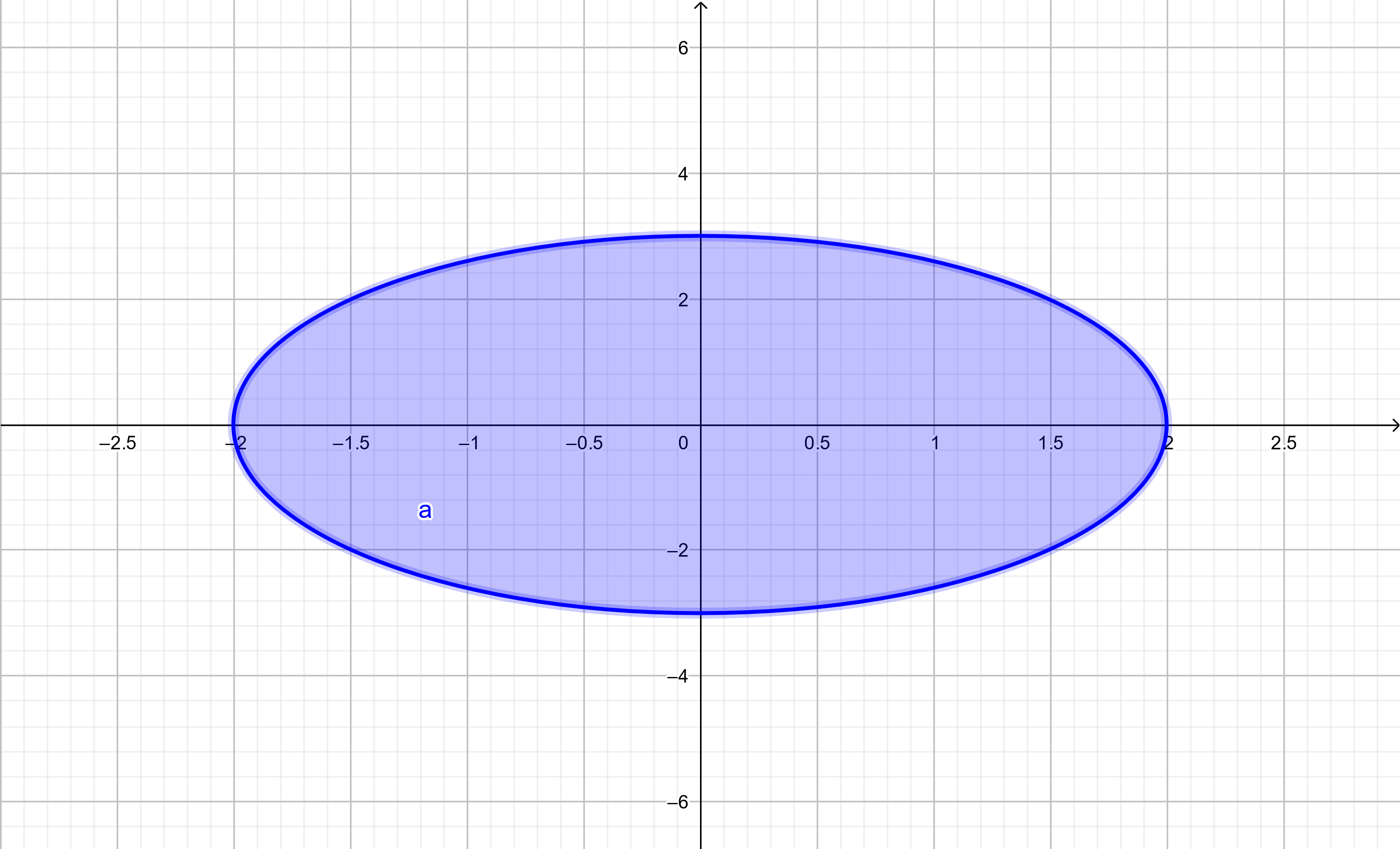Figure 5
We can use the entire real line as the codomain, The nonnegative real numbers $[0,\infty)$, or the image $[0,6]$.
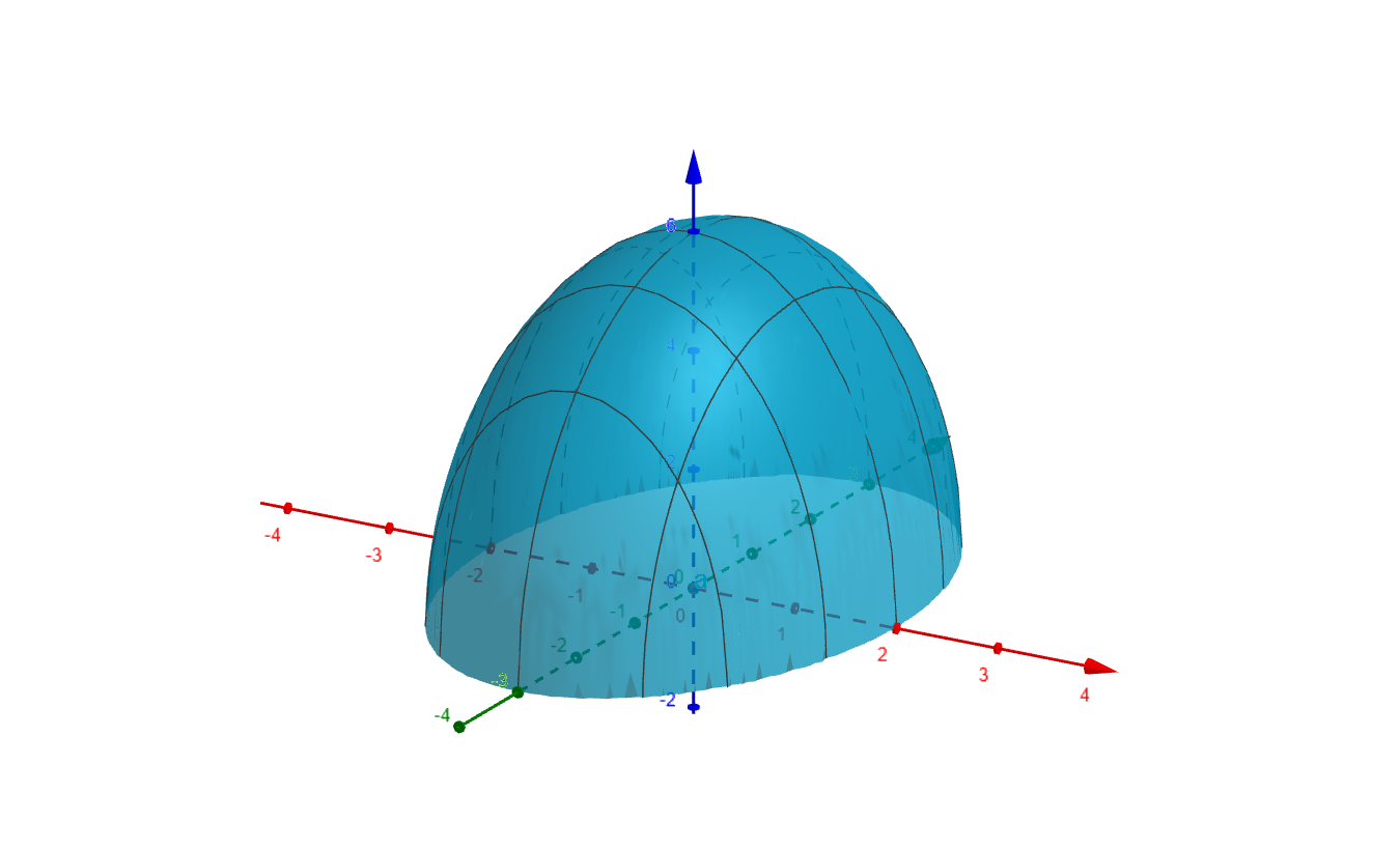Figure 6

14.1.5 Level Curves

One way to form a mental image of a surface or volume is using its level sets . Consider the graph

Figure 5

A level curve or contour of a function of two variables $z = f(x,y)$ is defined by the implicit function $f(x,y)=k$ for every real value $k$ in the image of $f$. A closed curve or several closed curves are formed as the intersection of the plane $z=k$. One may graph the curve of intersection of the surface and horizontal plane $z=k$ as in figure 1. The curves in the $xy$-plane are projections of the curves onto the plane.

14.1.6 Contour Plots

Typically one plots several cross section curves and their projections onto the $xy$-plane in one plot

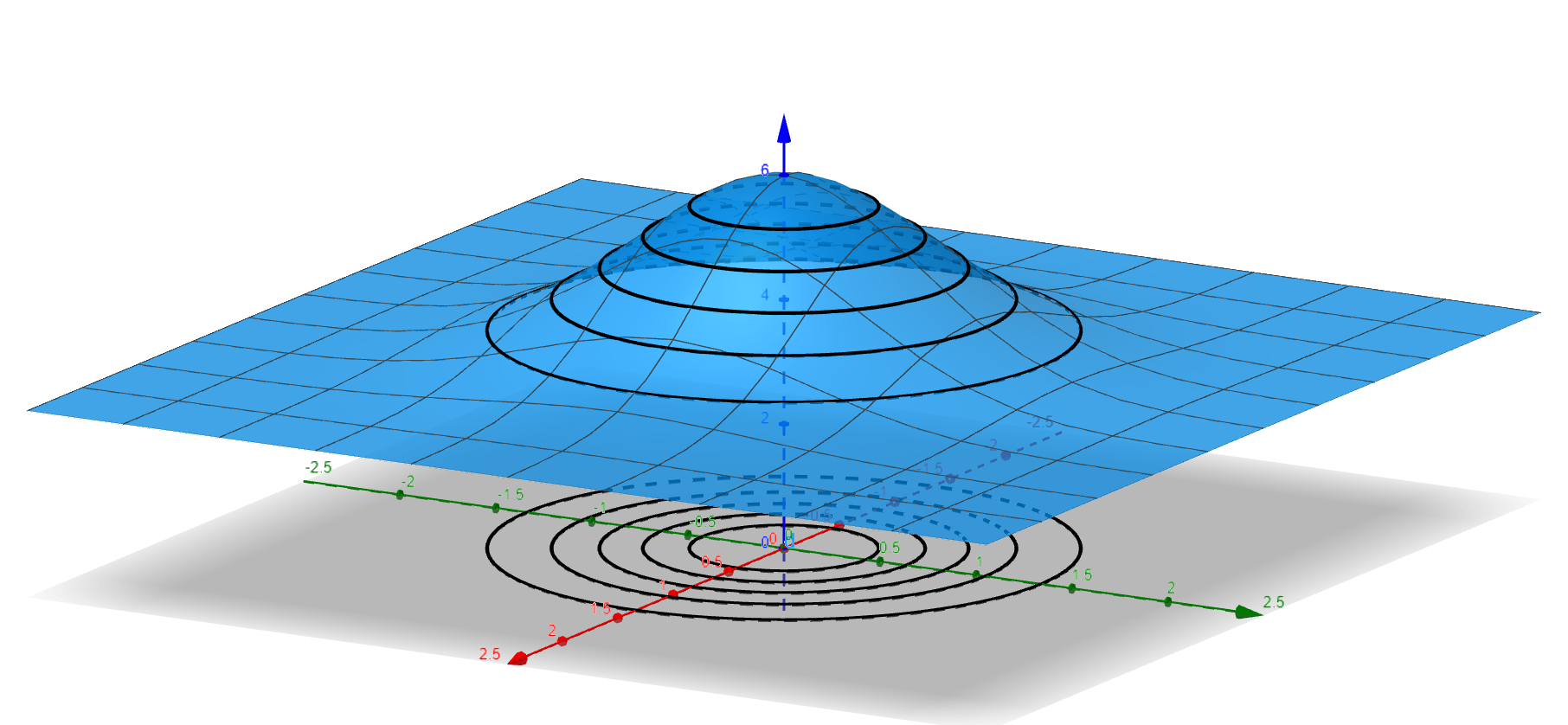
Figure 6

One creates a contour plot by graphing several level curves on the coordinate plane. Each equation

$$ 3\left(e^{-x^2-y^2}+1\right) = k $$
implicitly defines a function $y$ of $x$.

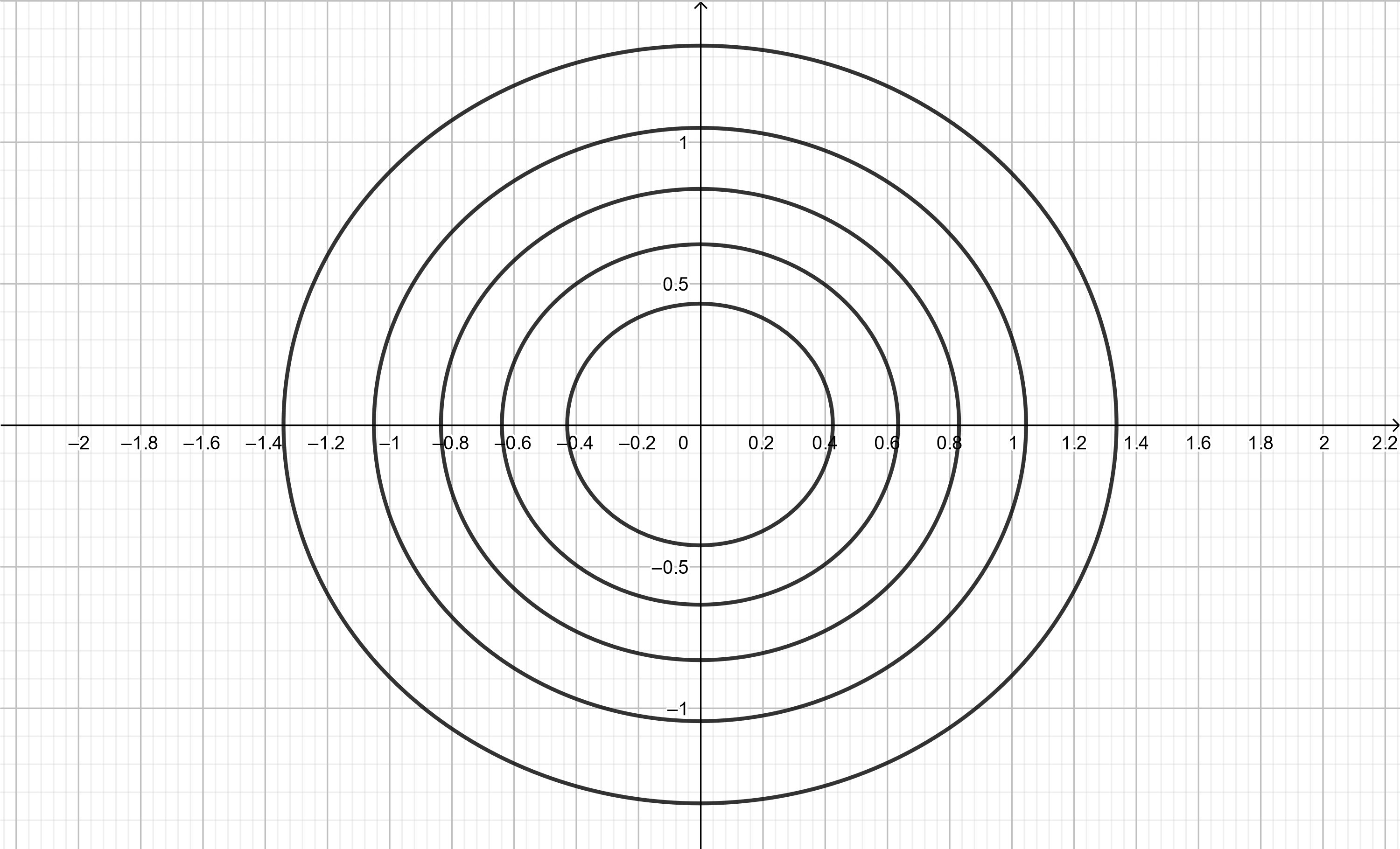Figure 7

If the vertical distance between values of $k$ are equal, one can infer steepness of the surface by the distance between level curves. When the curves are closer together, the surface is steeper. When the curves are farther apart, the surface is flatter.

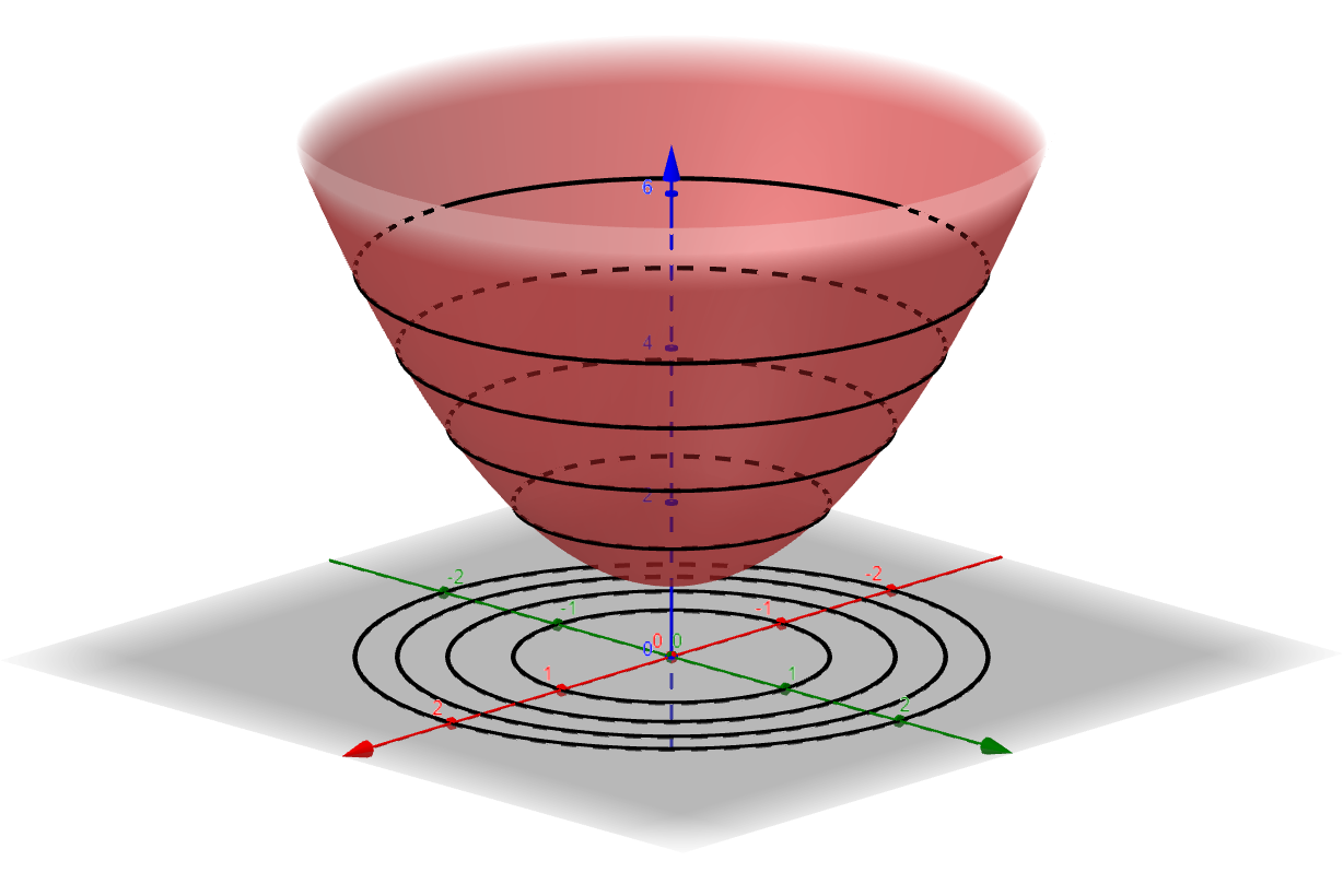Figure 8

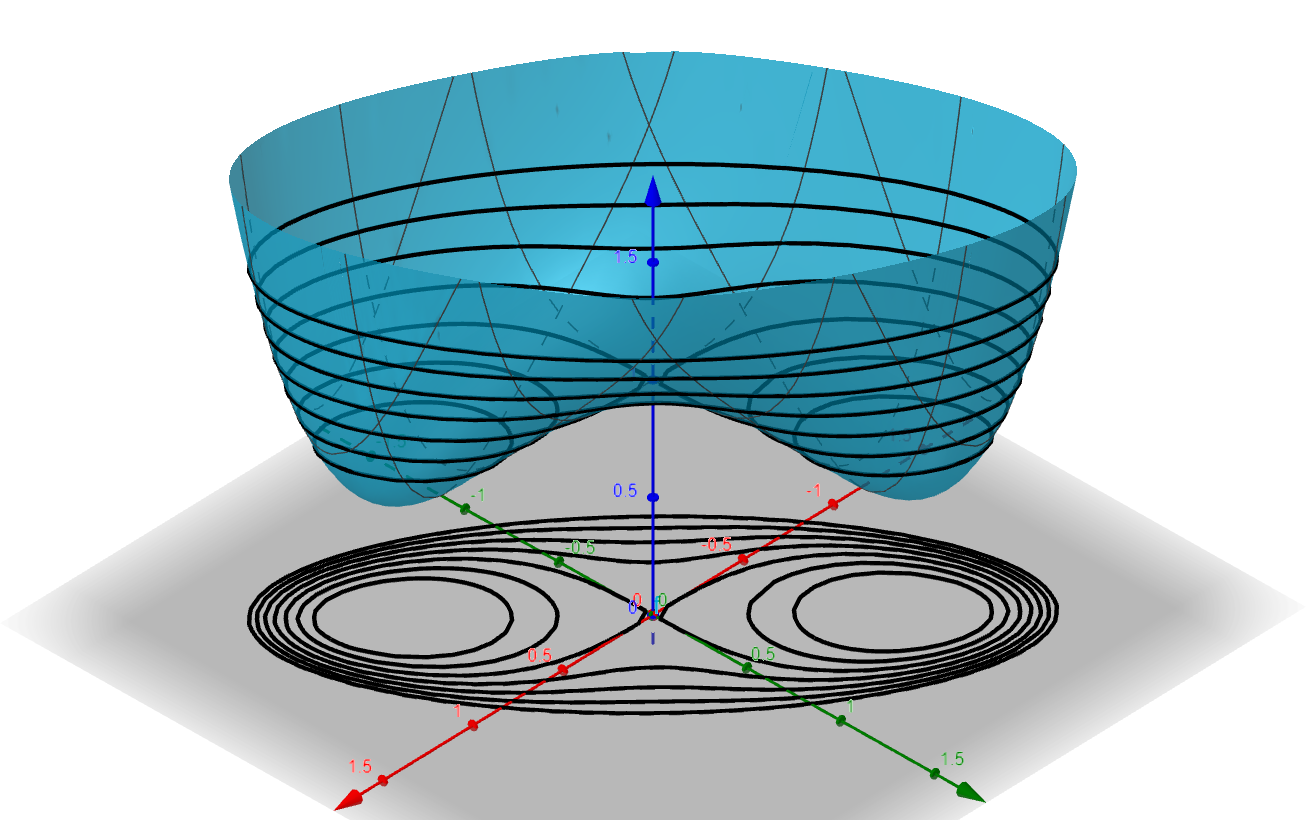Figure 9

Exercise 14.1.2

Consider the function $z = x^2 - 4y^2$

• Determine the domain of the function
  
  
• Determine the image of the function
  
  
• Determine an equation for the level sets $z=k$, for every $k$ in the image of our function.
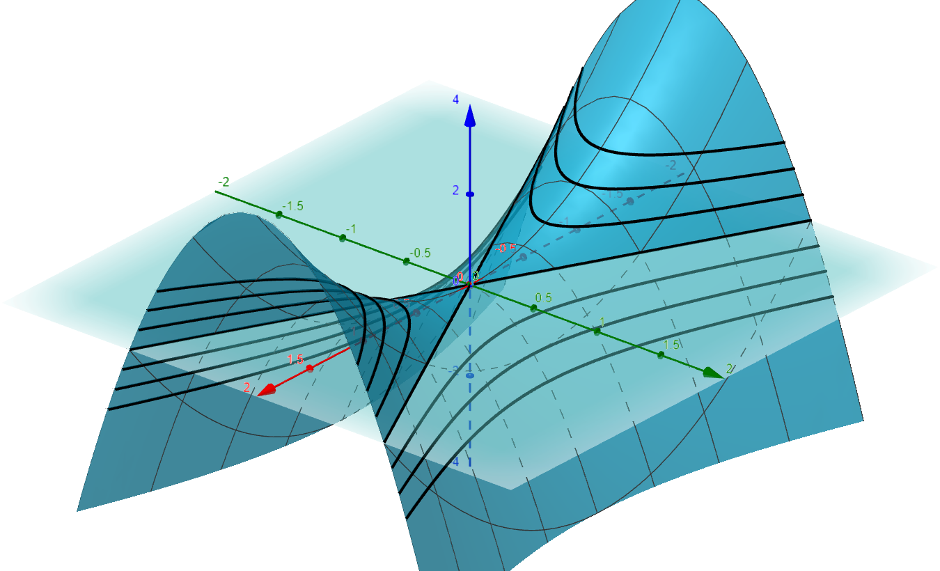  Figure 10
  
  

Check your work

* The domain of our function $z = f(x,y) = x^2 - 4y^2$ is the entire plane $\mathbb{R}^2$.
* The image of $f$ is the real line $\mathbb{R} = (-\infty,\infty)$.
* For any $k\in\mathbb{R}$ the equation of the level curve is given by
$$ x^2 - 4y^2 = k $$
The graph of these level curves are hyperbolas. A contour plot of our function for several values of $k$ 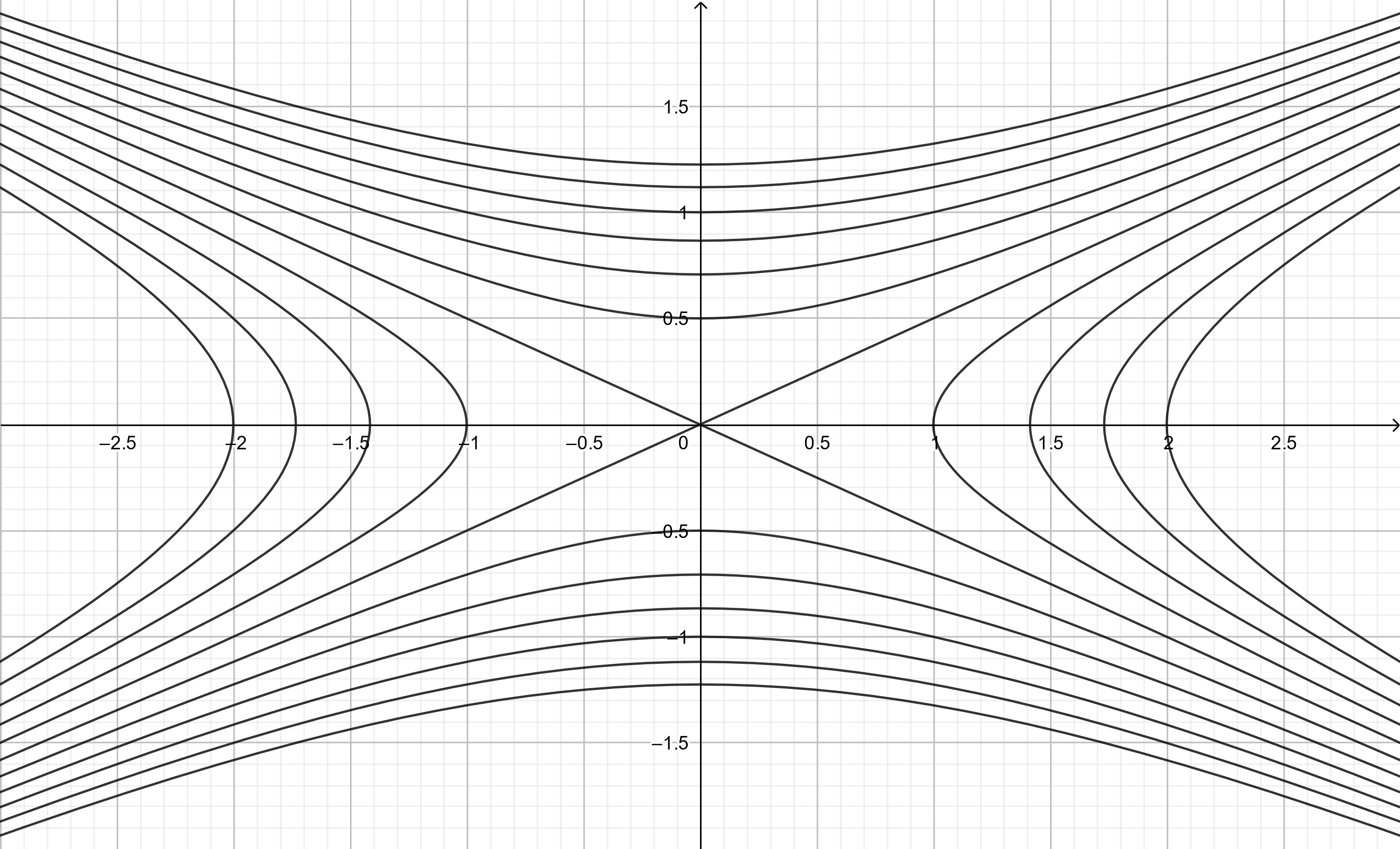Figure 11

14.1.7 Functions of Three Variables

A function $f$ of three variables assigns to each ordered triple $(x,y,z)$ in a volume $D\subset\mathbb{R}^3$ a unique real number $f(x,y,z)$. For example we could measure the temperature of $T$ at ever point in the atmosphere. This function for temperature depends on the longitude $x$, latitude $y$ and altitude $z$, so we write

$$ T = f(x,y,z) $$

Example 14.1.4

Consider the function defined by the equation

$$ w = \sqrt{49-x^2-y^2-z^2} $$
The reader must infer the domain and the codomain of the function $w = f(x,y,z) = \sqrt{49-x^2-y^2-z^2}$. Square root must have a nonnegative input and produces a nonnegative output. Thus to find the domain we have

$$ \begin{align*} 49-x^2-y^2-z^2 &\ge 0 \\ \\ x^2+y^2+z^2 &\le 49 \\ \end{align*} $$
The domain is the sphere of radius 7 centered at the origin

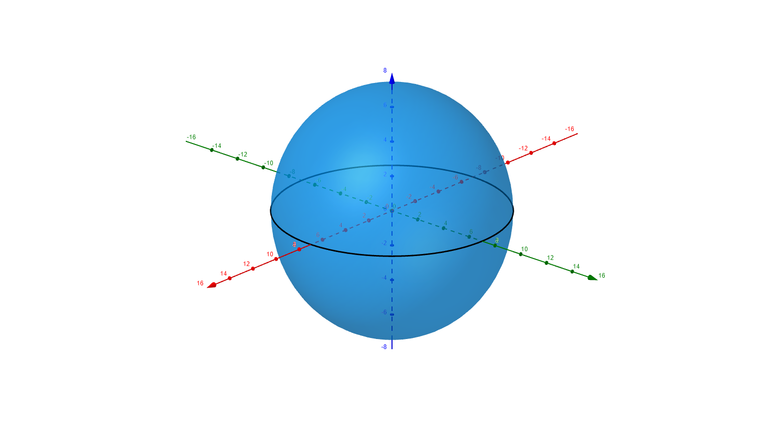Figure 12

Continuing one finds the image of function $f$

$$ \begin{align*} 0 \le x^2+y^2+z^2 &\le 49 \\ \\ 0 \le 49-x^2-y^2-z^2 &\le 49 \\ \\ 0 \le \sqrt{49-x^2-y^2-z^2} &\le 7 \\ \\ 0 \le f(x,y,z) &\le 7 \\ \end{align*} $$
The image of function $f$ is the interval $[0,7]$ on the real line $\mathbb{R}$. The graph of our function would require a four dimensional Euclidean space so we cannot represent it here. However we can graph the level sets of the function. For every real number $k$ in the image of $f$, $k\in[0,7]$, the level surface is described by the equation

$$ \begin{align*} \sqrt{49-x^2-y^2-z^2} &= k \\ \\ 49-x^2-y^2-z^2 &= k^2 \\ \\ x^2 + y^2 + z^2 &= 49 - k^2 \\ \end{align*} $$
The contour plot of our function for several values for $k$ yields level surfaces that are spheres of radius zero to seven.

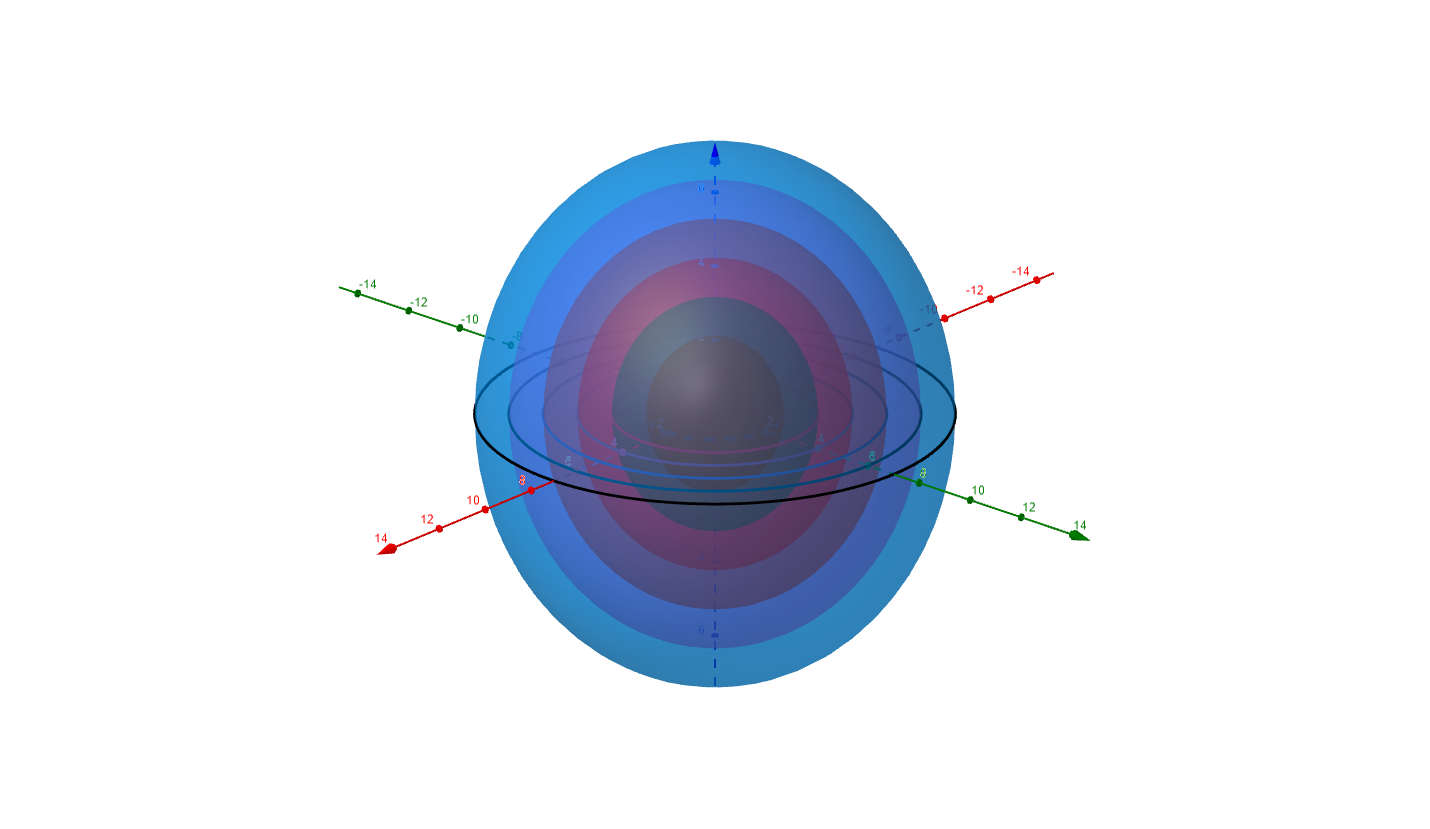Figure 13

Exercise 14.1.3

Consider function defined by the equation
$$ w = x^2 - \dfrac{y^2}{4} + z^2 $$

• Determine the domain and image of the function
  
  
• Determine the equation of the level surfaces
  
  
• Describe the level surfaces of the function
  
  

Check your work

* The domain of our function $w = f(x,y,z) = x^2 - \dfrac{y^2}{4} + z^2$ is all of three dimensional Euclidean space $\mathbb{R}^3$.
* The image of $f$ is the real line $\mathbb{R} = (-\infty,\infty)$.
* For any $k\in\mathbb{R}$ the equation of the level surface is given by

$$ x^2 - \dfrac{y^2}{4} + z^2 = k $$
The graph of these level surfaces are hyperboloids. A contour plot of our function for several values of $k$ 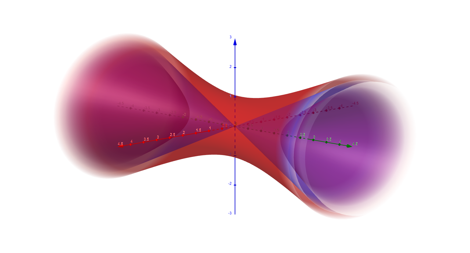Figure 14
The level surface is an hyperboloid with the $y$-axis as the axis of symmetry. The surface is a
* hyperboloid of one sheet if $k>0$
* cone if $k=0$
* hyperboloid of two sheets if $k<0$

14.1.8 Functions of Many Variables

A function $f$ of $n$ variables assigns to each ordered $n$-tuple $(x_1,x_2,x_3,\dots,x_n)$ in a volume $D\subset\mathbb{R}^n$ a unique real number $f(x_1,x_2,x_3,\dots,x_n)$.

For example chemometrics is used in analytical chemistry and other fields to solve predictive and quantification problems. Often combinations of infrared and UV/visible spectroscopy, mass spectrometry, nuclear magnetic resonance, atomic emission/absorption, and chromatography measurements are used as inputs to determine a single quantity or property. In many applications several or thousands of measurements are used to obtain an accurate result. The mathematical model consists of a multivariate function with many inputs and a single output.

In applications, analytical devices that combine the results of several detectors into a quantitative result must be calibrated from known samples and the mathematical models developed from chemometric analysis.

The social sciences, business, agriculture, and epidemiology also require mathematical models based on several, hundreds, or thousands of inputs to determine a useful result.

Data Science is a field that focuses on extracting useful information from typically very large data sets. While these functions can not be graphed in the sense of functions of one or two inputs, applied mathematicians and data scientists employ novel techniques to graphically represent multivariate functions. While we will limit most of our examples and exercises to functions with one to three inputs and outputs the student must remember that the techniques learned in this course apply equally well to functions with thousands of inputs and hundreds of outputs.

In this chapter we restrict ourselves to functions with one output and $n$ inputs for some positive integer $n$. Thus the domain of our functions are some subset of Euclidean space $\mathbb{R}^n$. If set $D\subset\mathbb{R}^n$ then we can define a function from $D$ to the real numbers

$$ f:D\rightarrow\mathbb{R} $$
and define our function as

• a function of $n$ real variables $x_1, x_2, \dots, x_n$, $y = f(x_1, x_2, \dots x_n)$;
  
  

• a function of a point in $\mathbb{R}^n$, $p = (x_1, x_2, \dots, x_n)\in\mathbb{R}^n$, $y = f(p)$;
  
  

• a function of a single vector $\mathbf{x} = \langle x_1, x_2, \dots, x_n\rangle\in\mathbb{R}^n$, $y = f(\mathbf{x})$;
  
  

All three viewpoints are useful.

Example 14.1.5

For a fixed vector $\mathbf{c}\in\mathbb{R}^n$ we can define a function $f:\mathbb{R}^n\rightarrow\mathbb{R}$ using dot product

$$ y = f(\mathbf{x}) := \mathbf{c}\cdot\mathbf{x}, $$
for every $\mathbf{x}\in\mathbb{R}^n$.

Your use of this self-initiated mediated course material is subject to our Creative Commons License .

Creative Commons Attribution-NonCommercial-ShareAlike 4.0


Attribution
You must give appropriate credit, provide a link to the license, and indicate if changes were made. You may do so in any reasonable manner, but not in any way that suggests the licensor endorses you or your use.


Noncommercial
You may not use the material for commercial purposes.


Share Alike
You are free to share, copy and redistribute the material in any medium or format. If you adapt, remix, transform, or build upon the material, you must distribute your contributions under the same license as the original.