Math 344: Calculus III

14.3 Partial Derivatives

---

14.3.1 The Tangent Plane to a Surface at a Point

A graph of a function $f$ of two variables yields a surface $ \require{color} \definecolor{brightblue}{rgb}{.267, .298, .812} \definecolor{darkblue}{rgb}{.08, .18, .28} \definecolor{palepink}{rgb}{1, .73, .8} \definecolor{softmagenta}{rgb}{.99,.34,.86} \def\ihat{\mathbf{\hat{\mmlToken{mi}[mathvariant="bold"]{ı}}}} \def\jhat{\mathbf{\hat{\mmlToken{mi}[mathvariant="bold"]{ȷ}}}} \def\khat{\mathbf{\hat{k}}} z = f(x,y) $. For each ordered pair $(x,y)$ on the $xy$-plane we have a single output or height.

The graph of $z = f(x,y) = 4 - \dfrac{x^2}{8} - \dfrac{y^2}{8}$
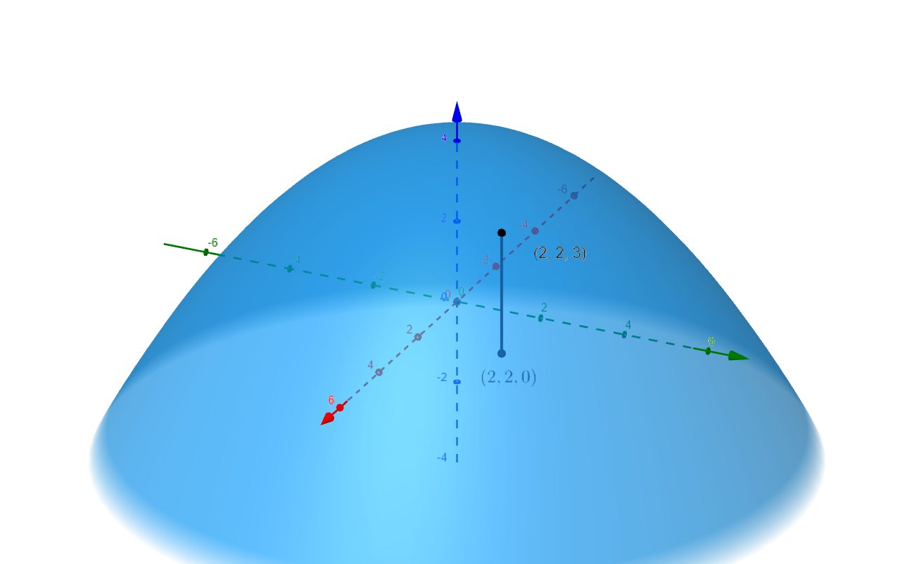
Figure 1

This surface is parameterized by two independent variables. We can describe the surface as the graph of




$$ \begin{align*} z &= f(x,y) = 4 - \dfrac{x^2}{8} - \dfrac{y^2}{8} &\qquad &\text{scalar equation} \\ \\ \mathbf{r}(x,y) &= \langle x, y, f(x,y)\rangle = \left\langle x,\ y,\ 4 - \dfrac{x^2}{8} - \dfrac{y^2}{8}\right\rangle &\qquad &\text{vector equation} \\ \\ x(u,v) &= u &\qquad &\text{parametric equations} \\ y(u,v) &= v \\ z(u,v) &= 4 - \dfrac{u^2}{8} - \dfrac{v^2}{8} \end{align*} $$

If we fix $x$, $y$, or $z$ we obtain a level curve on the surface. For example if we fix $y=2$, then we have the equation

$$ z = 4 - \dfrac{x^2}{8} - \dfrac{2^2}{8} = 3.5 - \dfrac{x^2}{8} $$
The graph of this parabola has the parametric equations

$$ \begin{align*} x &= t \\ \\ y &= 2 \\ z &= 3.5 - \dfrac{t^2}{8} \end{align*} $$

The Level Set $\mathbf{r}(t) = \left\langle t,\ 2,\ 3.5 - \dfrac{t^2}{8}\right\rangle$
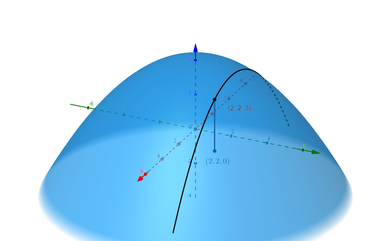
Figure 2

This curve is the intersection of the plane $y=2$ and the paraboloid. This level curve lies in a plane parallel to the $xz$-plane. This level curve is differentiable.

$$ \mathbf{r}'(t) = \left\langle 1,\ 0,\ 0 - \dfrac{t}{4} \right\rangle $$
We can use the velocity or derivative vector as the slope vector for the equation of the tangent line to the curve at each point on the curve. This will also be a tangent line for the surface at each point on the curve.

The Tangent Line at Each Point on the Level Curve
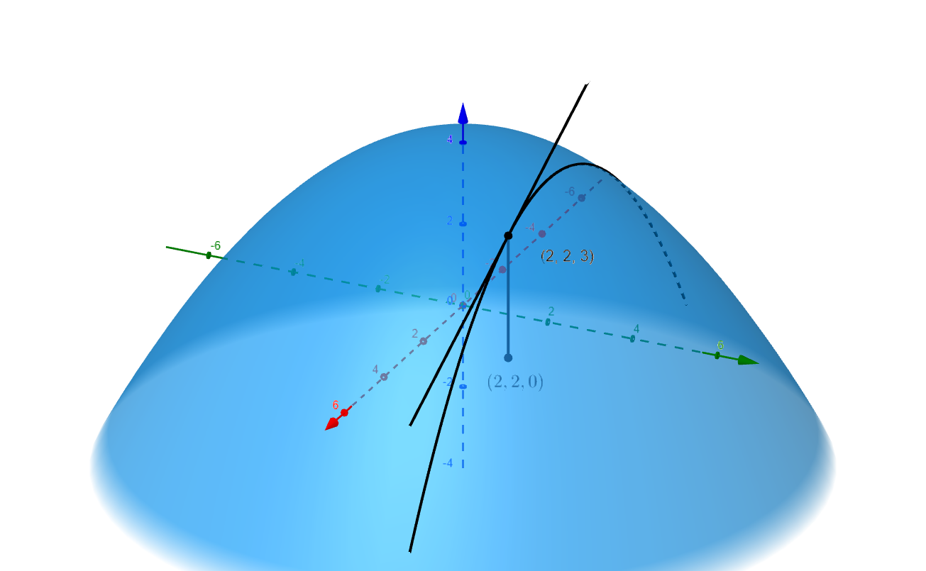
Figure 3

If we move the tail of the velocity vector to sit on our point $P(2,2,3)$, then we have a tangent vector at $P$, and on the tangent line.

A Tangent Vector at Each Point on the Level Curve
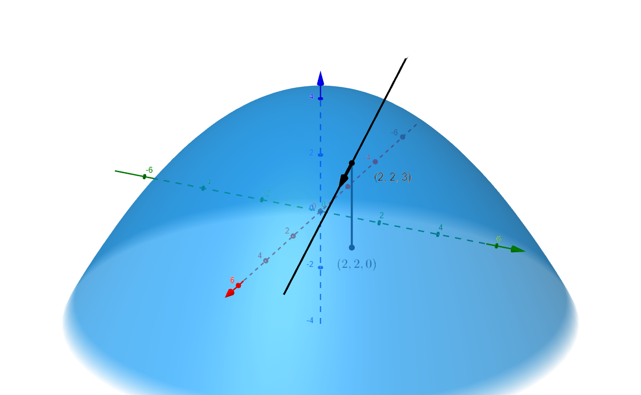
Figure 4

Likewise we get different level set in a plane parallel to the $yz$-plane setting $x=2$. The intersection of the plane $x=2$ and the paraboloid is a level curve parameterized by the equation

Another Level Curve on the Paraboloid
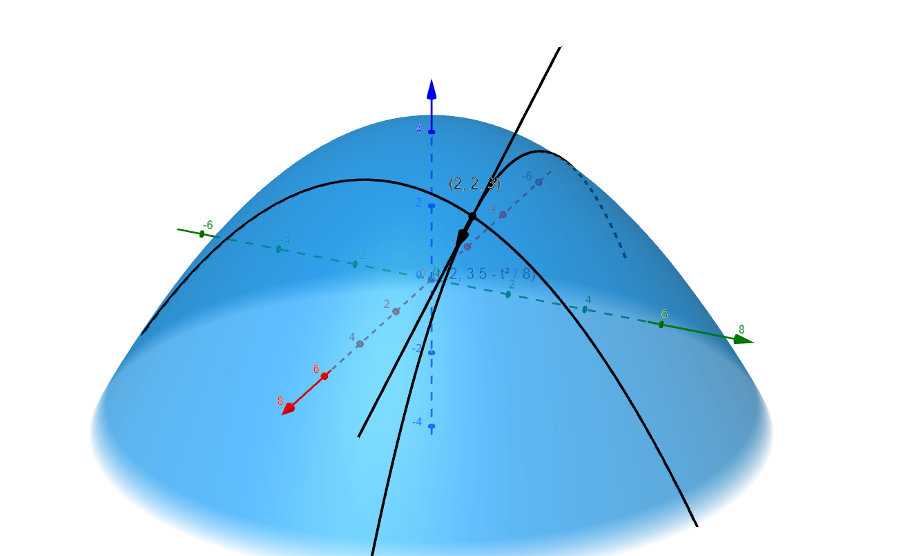
Figure 5

This level curve is also differentiable and has a velocity vector that we can use for the equation of the line.

Another Tangent Vector on the Paraboloid
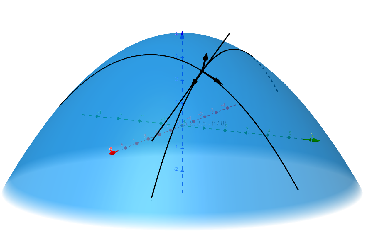
Figure 6

These two tangent vectors are not collinear as one is in a plane parallel to the $xz$-plane and one is in the plane parallel to the $yz$-plane. We learned earlier that the span of two vectors is a plane. The cross product of these two basis vectors is a mutually perpendicular normal vector we can use to describe the vector equation of the plane that intersects the surface at point $P$.

$$ \mathbf{n}\cdot\left(\mathbf{r}-\mathbf{\overrightarrow{OP}}\right) = 0; $$

The Tangent Plane on the Paraboloid
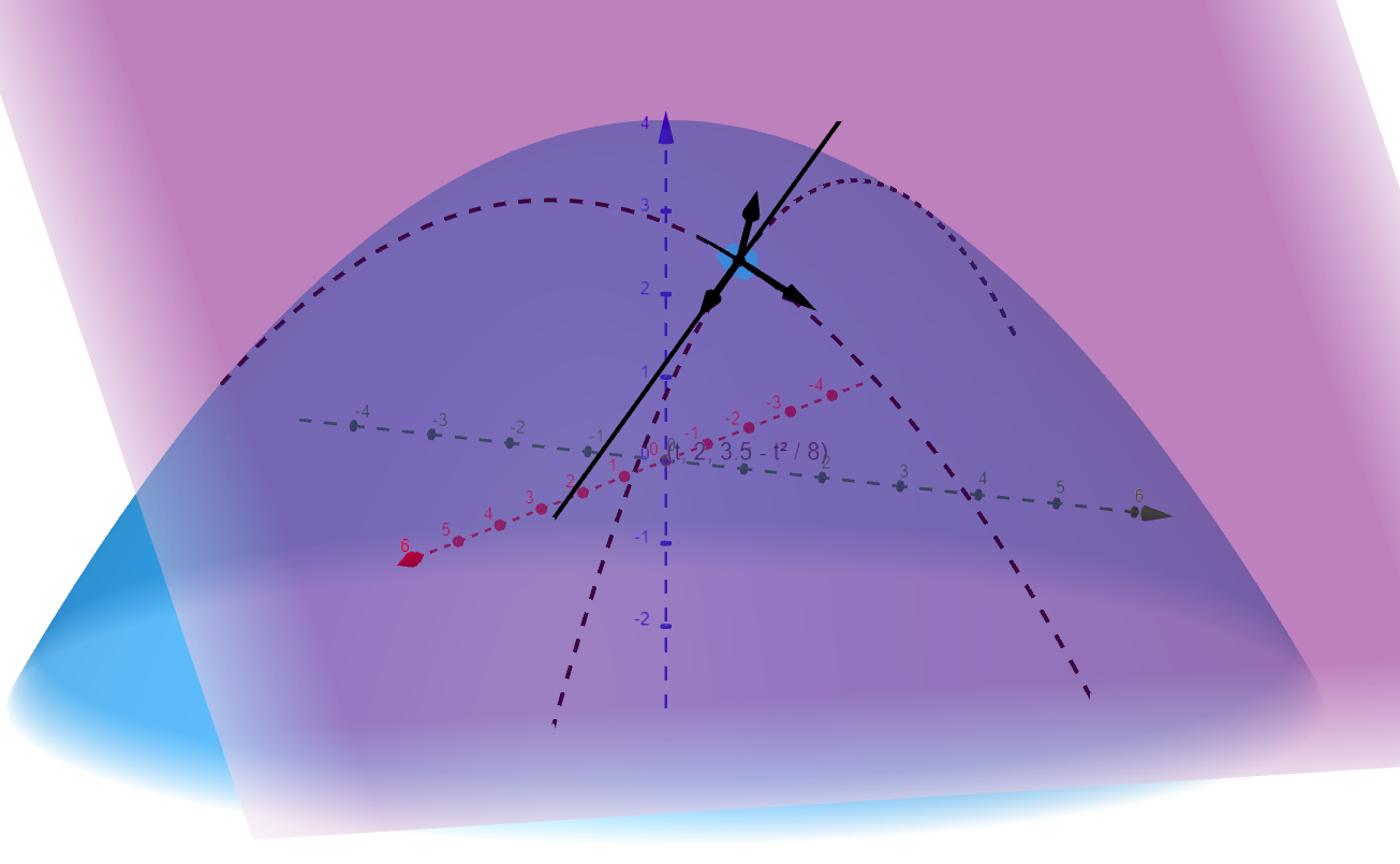
Figure 7

14.3.2 Computing Partial Derivatives

We need a method of computing the slope of the tangent line to each of the level curves. In our previous example we chose the level curve setting $y=2$, yielding

$$ z = g(x) := f(x,2) = 4 - \dfrac{x^2}{8} - \dfrac{2^2}{8} = \dfrac{32-4}{8} - \dfrac{x^2}{8} = \dfrac{28-x^2}{8} $$
This results in a curve parameterized by the equation

$$ \mathbf{r}(x) = \left\langle x, 2, g(x) \right\rangle = \left\langle x, 2, \dfrac{28-x^2}{8} \right\rangle $$
We are interested in the velocity vector at the point $P(2,2,3)$, or

$$ \mathbf{r}(2) = \left\langle 2, 2, \dfrac{28-2^2}{8} \right\rangle = \langle 2, 2, 3\rangle = \mathbf{\overrightarrow{0P}}. $$
The velocity vector at $P$ is computed in chapter 13 as

$$ \mathbf{r}'(2) = \left.\left\langle 1, 2, \dfrac{0-2x}{8} \right\rangle\right|_{x=2} = \left\langle 1, 2, -\dfrac{4}{8} \right\rangle = \left\langle 1, 2, -\dfrac{1}{2} \right\rangle $$

In fact for any fixed but arbitrary value ${\color{softmagenta}y}$,
$$ \begin{align*} \mathbf{r}'(x) &:= \dfrac{d}{dx}\left\langle x, {\color{softmagenta}y}, f(x,{\color{softmagenta}y}) \right\rangle \\ \\ &= \dfrac{d}{dx}\left\langle x, {\color{softmagenta}y}, g(x) \right\rangle \\ \\ &= \left\langle 1, {\color{softmagenta}y}, g'(x) \right\rangle \end{align*} $$

Usually we realize that the second variable is fixed . We call computing the derivative with the second variable fixed the partial derivative of $\mathbf{f}$ with respect to the first variable . Partial Derivatives compute the limit of the difference quotient with respect to one input variable, considering all other input variables to the constants. The symbol for a partial derivative $\partial$ used today in Leibniz notation was reintroduced by Carl Gustav Jacob Jacobi in 1841. The Newton notation for a partial derivative is to indicate the derivative variable in a subscript.

$$ \begin{align*} D_1\,f(x,y) &= f_1({\color{softmagenta}x},y) = D_{\color{softmagenta}x}\,f(x,y) = f_{\color{softmagenta}x}({\color{softmagenta}x},y) &\qquad &\text{Newtonian notation} \\ \\ &= \dfrac{\partial f}{\partial {\color{softmagenta}x}}({\color{softmagenta}x},y) = \dfrac{\partial}{\partial{\color{softmagenta}x}}f({\color{softmagenta}x},y) &\qquad &\text{Leibniz notation} \\ \\ &:= \displaystyle\lim_{{\color{softmagenta}h}\rightarrow 0} \dfrac{f({\color{softmagenta}x+h},y) - f({\color{softmagenta}x},y)}{\color{softmagenta}h} &\qquad &\text{Definition} \end{align*} $$

The velocity vector to the level curve intersection of the surface $z=f(x,y)$ and a plane parallel to the $xz$-plane of the vector function $\mathbf{r}(x,y) = \langle x, y, f(x,y) \rangle$ is the vector

$$ \mathbf{r}_x(x,y) = \dfrac{\partial\,\mathbf{r}}{\partial x} = \left\langle 1, 0, \dfrac{\partial f}{\partial x} \right\rangle $$

Using this definition of the partial derivative with respect to $x$, we simply differentiate the expression for our function $f$ with respect to $x$ as if the value of $y$ is a constant.

Likewise, the definition of the partial derivative with respect to the second variable

$$ \begin{align*} D_2\,f(x,y) &= f_2(x,{\color{softmagenta}y}) = f_{\color{softmagenta}y}(x,{\color{softmagenta}y}) &\qquad &\text{Newtonian notation} \\ \\ &= \dfrac{\partial f}{\partial {\color{softmagenta}y}}(x,{\color{softmagenta}y}) = \dfrac{\partial}{\partial {\color{softmagenta}y}}f(x,{\color{softmagenta}y}) &\qquad &\text{Leibniz notation} \\ \\ &:= \displaystyle\lim_{{\color{softmagenta}h}\rightarrow 0} \dfrac{f(x,{\color{softmagenta}y+h}) - f(x,{\color{softmagenta}y})}{{\color{softmagenta}h}} \end{align*} $$

The velocity vector to the level curve intersection of the surface $z=f(x,y)$ and a plane parallel to the $yz$-plane is the vector

$$ \mathbf{r}_y(x,y) = \dfrac{\partial\,\mathbf{r}}{\partial y} = \left\langle 0, 1, \dfrac{\partial f}{\partial y} \right\rangle $$

Using the definition of the partial derivative with respect to $y$, we differentiate the expression for the function with respect to $y$ as if the value of $x$ is a constant.

14.3.3 Practice Computing Partial Derivatives

Example 14.3.1

Here is a table featuring several computed partial derivatives. Make sure that you follow along and agree with the calculations. Also, there are several different ways to indicate partial derivatives shown on the table. You will see all of them if you study different texts or resources. Start getting used to them.

Function	Partial Derivative
$f(x,y) = 36 - 9x^2 - 4y^2$	$f_1(x,y) = 36 - 18x$
	$f_2(x,y) = 36 - 8y$
$g(x,y) = 4xe^{xy^2}$	$g_x(x,y) = 4e^{xy^2} + 4xy^2e^{xy^2}$
	$g_y(x,y) = 4x\left(2xye^{xy^2}\right) = 8x^2ye^{xy^2}$
$h(u,v) = u\ln\left(uv + v^2\right)$	$\dfrac{\partial h}{\partial u} = \ln\left(uv + v^2\right) + u\dfrac{v}{uv + v^2} = \ln\left(uv + v^2\right) + \dfrac{u}{u + v}$
	$\dfrac{\partial h}{\partial v} = u\dfrac{u + 2v}{uv + v^2} = \dfrac{2uv + u^2}{uv + v^2}$
$F(r,\theta) = \left\langle r\cos(\theta), r\sin(\theta), r^2\right\rangle$	$\dfrac{\partial F}{\partial r} = \left\langle \cos(\theta), \sin(\theta), 2r\right\rangle$
	$F_{\theta} = \left\langle -r\sin(\theta), r\cos(\theta), 0 \right\rangle$

Exercise 14.3.1

Determine the indicated partial derivative of each function

Function	Partial Derivative
$1.\quad f(x,y) = 3x^4y^3 - e^xy^2 + 4y - x^{13}$	$f_x$
$2.\quad w = \cos\left(u^2 + 4v\right) - e^{3u-u^3v^2} + v^3$	$\dfrac{\partial w}{\partial v}$
$3.\quad R(x,y) = \dfrac{x^2}{x^2 + y^2} - \dfrac{y^2}{x^2 + y^2}$	$R_y$
$4.\quad x^2\sin(y^2) + xe^{3z} - \cos(z) = 2y + 6z - 4$	$\dfrac{\partial z}{\partial x}$

Check your work

1.

$$ f_x = 12x^3y^3 - e^xy^2 - 13x^{12} $$
2.

$$ \begin{align*} \dfrac{\partial w}{\partial v} &= -\sin\left(u^2 + 4v\right)\left(0 + 4\right) - e^{3u-u^3v^2}\left(0 - 2u^3v\right) + 3v^2 \\ \\ &= -4\sin\left(u^2 + 4v\right) + 2u^3ve^{3u-u^3v^2} + 3v^2 \end{align*} $$
3.

$$ \begin{align*} R_y &= -\dfrac{x^2}{\left(x^2 + y^2\right)^2}(2y) - \dfrac{2y\left(x^2 + y^2\right)- y^2(2y)}{\left(x^2 + y^2\right)^2} \\ \\ &= \dfrac{-2x^2y}{\left(x^2 + y^2\right)^2} - \dfrac{2x^2y + 2y^3- 2y^3}{\left(x^2 + y^2\right)^2} \\ \\ &= -\dfrac{4x^2y}{\left(x^2 + y^2\right)^2} \end{align*} $$
4.

$$ \begin{align*} \dfrac{\partial}{\partial x}\left(x^2\sin(y^2) + xe^{3z} - \cos(z)\right) &= \dfrac{\partial}{\partial x}\left( 2y + 6z - 4 \right) \\ \\ 2x\sin(y^2) + e^{3z} + 3xe^{3z}\dfrac{\partial z}{\partial x} + \sin(z)\dfrac{\partial z}{\partial x} &= 0 + 6\dfrac{\partial z}{\partial x} - 0 \\ \\ 2x\sin(y^2) + e^{3z} &= 6\dfrac{\partial z}{\partial x} - 3xe^{3z}\dfrac{\partial z}{\partial x} - \sin(z)\dfrac{\partial z}{\partial x} \\ \\ \dfrac{\partial z}{\partial x}\left(6 - 3xe^{3z} - \sin(z)\right) &= 2x\sin(y^2) + e^{3z} \\ \\ \dfrac{\partial z}{\partial x} &= \dfrac{2x\sin(y^2) + e^{3z}}{6 - 3xe^{3z} - \sin(z)} \end{align*} $$

Now try to compute the partial derivatives not listed in the table. Results are presented in this video example:

Video Solution

14.3.5 Higher Order Derivatives

A function $z = f(x,y)$ defined with two inputs will have two first order derivatives

$$ \begin{align*} z_x &= f_x = \dfrac{\partial z}{\partial x} = \dfrac{\partial f}{\partial x} \\ \\ z_y &= f_y = \dfrac{\partial z}{\partial y} = \dfrac{\partial f}{\partial y} \end{align*} $$
However this function has four second order derivatives. This is due to that fact that higher order derivatives are compositions of differential operators. In Newtonian notation, the order of the derivatives are listed in the subscripts. Thus the derivative of $f_x$ with respect to $y$ is $f_{xy}$. However in Leibniz notation we see the composition of derivatives

$$ f_{xy} = \dfrac{\partial}{\partial y}\left(\dfrac{\partial}{\partial x}\,f\right) = \dfrac{\partial^2 f}{\partial y\partial x} $$

Second Derivative	$\dfrac{\partial}{\partial x}$	$\dfrac{\partial}{\partial y}$
$\color{softmagenta}\dfrac{\partial}{\partial x}$	$z_{x{\color{softmagenta}x}} = f_{x{\color{softmagenta}x}} = \dfrac{\partial^{\color{softmagenta}2} z}{\partial x^{\color{softmagenta}2}} = \dfrac{\partial^{\color{softmagenta}2} f}{\partial x^{\color{softmagenta}2}}$	$z_{y{\color{softmagenta}x}} = f_{y{\color{softmagenta}x}} = \dfrac{\partial^{\color{softmagenta}2} z}{{\color{softmagenta}\partial x}\partial y} = \dfrac{\partial^{\color{softmagenta}2} f}{{\color{softmagenta}\partial x}\partial y}$
$\color{softmagenta} \dfrac{\partial}{\partial y}$	$z_{x{\color{softmagenta}y}} = f_{x{\color{softmagenta}y}} = \dfrac{\partial^{\color{softmagenta}2} z}{{\color{softmagenta}\partial y}\partial x} = \dfrac{\partial^{\color{softmagenta}2} f}{{\color{softmagenta}\partial y}\partial x}$	$z_{y{\color{softmagenta}y}} = f_{y{\color{softmagenta}y}} = \dfrac{\partial^{\color{softmagenta}2} z}{\partial y^{\color{softmagenta}2}} = \dfrac{\partial^{\color{softmagenta}2} f}{\partial y^{\color{softmagenta}2}}$

Likewise a function with two inputs will have eight third order partial derivatives

$$ \begin{array}{lcl} f_{xxx} = \dfrac{\partial}{\partial x}\dfrac{\partial}{\partial x}\dfrac{\partial}{\partial x}f = \dfrac{\partial^3 f}{\partial x^3} & \quad & f_{xxy} = \dfrac{\partial}{\partial y}\dfrac{\partial}{\partial x}\dfrac{\partial}{\partial x}f = \dfrac{\partial^3 f}{\partial y\partial x^2} \\ f_{xyx} = \dfrac{\partial}{\partial x}\dfrac{\partial}{\partial y}\dfrac{\partial}{\partial x}f = \dfrac{\partial^3 f}{\partial x\partial y\partial x} & \quad & f_{xyy} = \dfrac{\partial}{\partial y}\dfrac{\partial}{\partial y}\dfrac{\partial}{\partial x}f = \dfrac{\partial^3 f}{\partial^2 y\partial x} \\ f_{yxx} = \dfrac{\partial}{\partial x}\dfrac{\partial}{\partial x}\dfrac{\partial}{\partial y}f = \dfrac{\partial^3 f}{\partial x^2\partial y} & \quad & f_{yxy} = \dfrac{\partial}{\partial y}\dfrac{\partial}{\partial x}\dfrac{\partial}{\partial y}f = \dfrac{\partial^3 f}{\partial y\partial x\partial y} \\ f_{yyx} = \dfrac{\partial}{\partial x}\dfrac{\partial}{\partial y}\dfrac{\partial}{\partial y}f = \dfrac{\partial^3 f}{\partial x\partial y^2} & \quad & f_{yyy} = \dfrac{\partial}{\partial y}\dfrac{\partial}{\partial y}\dfrac{\partial}{\partial y}f = \dfrac{\partial^3 f}{\partial y^3} \end{array} $$

14.3.6 Clairaut's Theorem

Theorem 14.3.6

Clairaut's Theorem
If the two mixed, second order partial derivatives of a function defined on an open disk in the plane $D\subset\mathbb{R}^2$ are both continuous on the disk $D$, then they are equal on $D$:

$$ f_{xy} = f_{yx}. $$

A higher order derivative is called mixed if it involves partial derivatives with respect to more than one input. Hence $f_{xx}$ and $f_{yy}$ are not mixed partial derivatives. To use Clairaut's Theorem to assert that the two mixed, second order partial derivatives are equal at a point $(x_0,y_0)$, they must both be continuous on some disk of radius $r>0$ centered at the point $(x_0,y_0)$.

Example 14.3.2

Consider the function described by the equation

$$ z = x^3y^2 - \dfrac{4y^6}{x^3} $$
The two first order derivatives are

$$ \begin{align*} \dfrac{\partial z}{\partial x} &= 3x^2y^2 + \dfrac{12y^6}{x^4} \\ \\ \dfrac{\partial z}{\partial y} &= 2x^3y - \dfrac{24y^5}{x^3} \\ \end{align*} $$
The four second order derivatives are

$$ \begin{array}{lcl} \dfrac{\partial^2 z}{\partial x^2} = 6xy^2 - \dfrac{48y^6}{x^5} & \quad & \dfrac{\partial^2 z}{\partial y\partial x} = 6x^2y + \dfrac{72y^5}{x^4} \\ \dfrac{\partial^2 z}{\partial x\partial y} = 6x^2y + \dfrac{72y^5}{x^4} & \quad & \dfrac{\partial^2 z}{\partial y^2} = 2x^3 - \dfrac{120y^4}{x^3} \end{array} $$
Notice that Clairaut's Theorem holds for every point on the plane $\mathbb{R}^2$ except the points where $x=0$. None of the second order partial derivatives have a value when $x=0$.

14.3.7 Practice Using Clairaut's Theorem

Exercise 14.3.2

Find all second order derivatives of the following functions and verify Clairaut's Theorem if the hypotheses of the theorem are met.

$$ \begin{align*} 1.&\quad g(u,v) = u^4v^2 - 2uv^{2/3} - \cos(3u) \\ \\ 2.&\quad f(x,y,z) = x^2y^3 - 2x^3z + 8y^3z^2 + z^3 \\ \\ 3.&\quad h(s,t) = s^2e^t + \ln(t - s) \end{align*} $$

Check your work

1. $$ \begin{align*} g_u &= 4u^3v^2 - 2v^{2/3} + 3\sin(3u) \\ \\ g_v &= 2u^4v - \dfrac{4}{3}uv^{-1/3} \end{align*} $$
$$ \begin{align*} g_{uu} &= 12u^2v^2 + 9\cos(3u) &\qquad g_{uv} &= 8u^3v - \dfrac{4}{3}v^{-1/3} \\ \\ g_{vu} &= 8u^3v - \dfrac{4}{3}v^{-1/3} &\qquad g_{vv} &= 2u^4 + \dfrac{4}{9}uv^{-4/3} \end{align*} $$
2. $$ \begin{align*} f_x &= 2xy^3 - 6x^2z \\ \\ f_y &= 3x^2y^2 + 24y^2z^2 \\ \\ f_z &= -2x^3 + 16y^3z + 3z^2 \\ \end{align*} $$
$$ \begin{align*} f_{xx} &= 2y^3 - 12xz &\qquad f_{yx} &= 6xy^2 &\qquad f_{zx} &= -6x^2 \\ \\ f_{xy} &= 6xy^2 &\qquad f_{yy} &= 6x^2y + 48yz^2 &\qquad f_{zy} &= 48y^2z \\ \\ f_{xz} &= -6x^2 &\qquad f_{yz} &= 48y^2z &\qquad f_{zz} &= 16y^3 + 6z \\ \end{align*} $$
3. $$ \begin{align*} h_s &= 2se^t - \dfrac{1}{t-s} \\ \\ h_t &= s^2e^t + \dfrac{1}{t-s} \\ \end{align*} $$
$$ \begin{align*} h_{ss} &= 2e^t - \dfrac{1}{(t-s)^2} &\qquad h_{st} &= 2se^t + \dfrac{1}{(t-s)^2} \\ \\ h_{ts} &= 2se^t + \dfrac{1}{(t-s)^2} &\qquad h_{tt} &= s^2e^t - \dfrac{1}{(t-s)^2} \\ \end{align*} $$

Your use of this self-initiated mediated course material is subject to our Creative Commons License .

Creative Commons Attribution-NonCommercial-ShareAlike 4.0


Attribution
You must give appropriate credit, provide a link to the license, and indicate if changes were made. You may do so in any reasonable manner, but not in any way that suggests the licensor endorses you or your use.


Noncommercial
You may not use the material for commercial purposes.


Share Alike
You are free to share, copy and redistribute the material in any medium or format. If you adapt, remix, transform, or build upon the material, you must distribute your contributions under the same license as the original.