Math 344: Calculus III

15.3 Double Integrals in Polar Coordinates

---

15.3.1 Polar Regions

The Definite integral from our first semester of calculus is a limit of Riemann Sums .

Polar Regions

Disk	Annulus	Annular Sector (Polar Rectangle)

Figure 1

Some regions on the plane just can't be easily described using functions of rectangular coordinates.

In single variable calculus we studied polar functions or function of polar coordinates

$$ \require{color} \definecolor{brightblue}{rgb}{.267, .298, .812} \definecolor{darkblue}{rgb}{.08, .18, .28} \definecolor{palepink}{rgb}{1, .73, .8} \definecolor{softmagenta}{rgb}{.99,.34,.86} \definecolor{brickred}{rgb}{.804,.12,.109} \def\ihat{\mathbf{\hat{\mmlToken{mi}[mathvariant="bold"]{ı}}}} \def\jhat{\mathbf{\hat{\mmlToken{mi}[mathvariant="bold"]{ȷ}}}} \def\khat{\mathbf{\hat{k}}} \newcommand{\pypx}[2][x]{\dfrac{\partial #2}{\partial #1}} \newcommand{\dydx}[2][x]{\dfrac{d #2}{d #1}} \newcommand{\deltax}[2][x]{\frac{\Delta #2}{\Delta #1}} x = r\cos(\theta)\qquad\qquad y = r\sin(\theta) $$

Example 1

The circle of radius one centered at the origin has rectangular equation

$$ x^2 + y^2 = 1 $$
and polar equation

$$ 1 = x^2 + y^2 = (r\cos(\theta))^2 + (r\sin(\theta))^2 = r^2\left(\cos^2(\theta) + \sin^2(\theta)\right) = r^2 $$
In polar coordinates $r$ represents the distance of from the origin to the tip of a vector and $\theta$ represents the angle the vector makes with the positive horizontal axis. Thus $r \ge 0$. The polar equation for the unit circle is given by

$$ r = 1 $$

Example 2

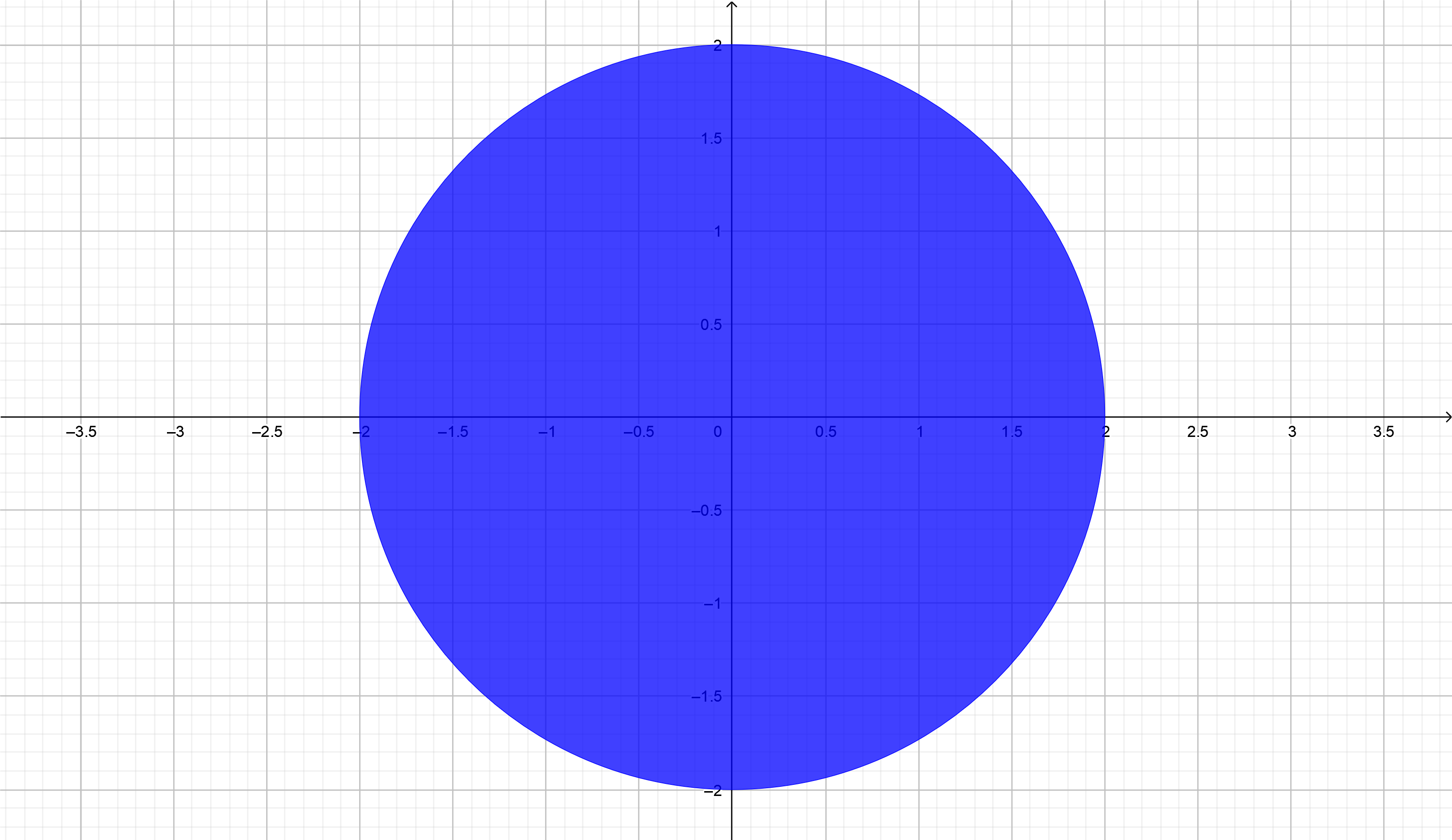
The unit disk of radius one centered at the origin is the locus of all points satisfying the rectangular equation

$$ x^2 + y^2 \le 1 $$
however the polar equation of the unit disk centered at the origin is given by

$$ r \le 1 $$

Example 3

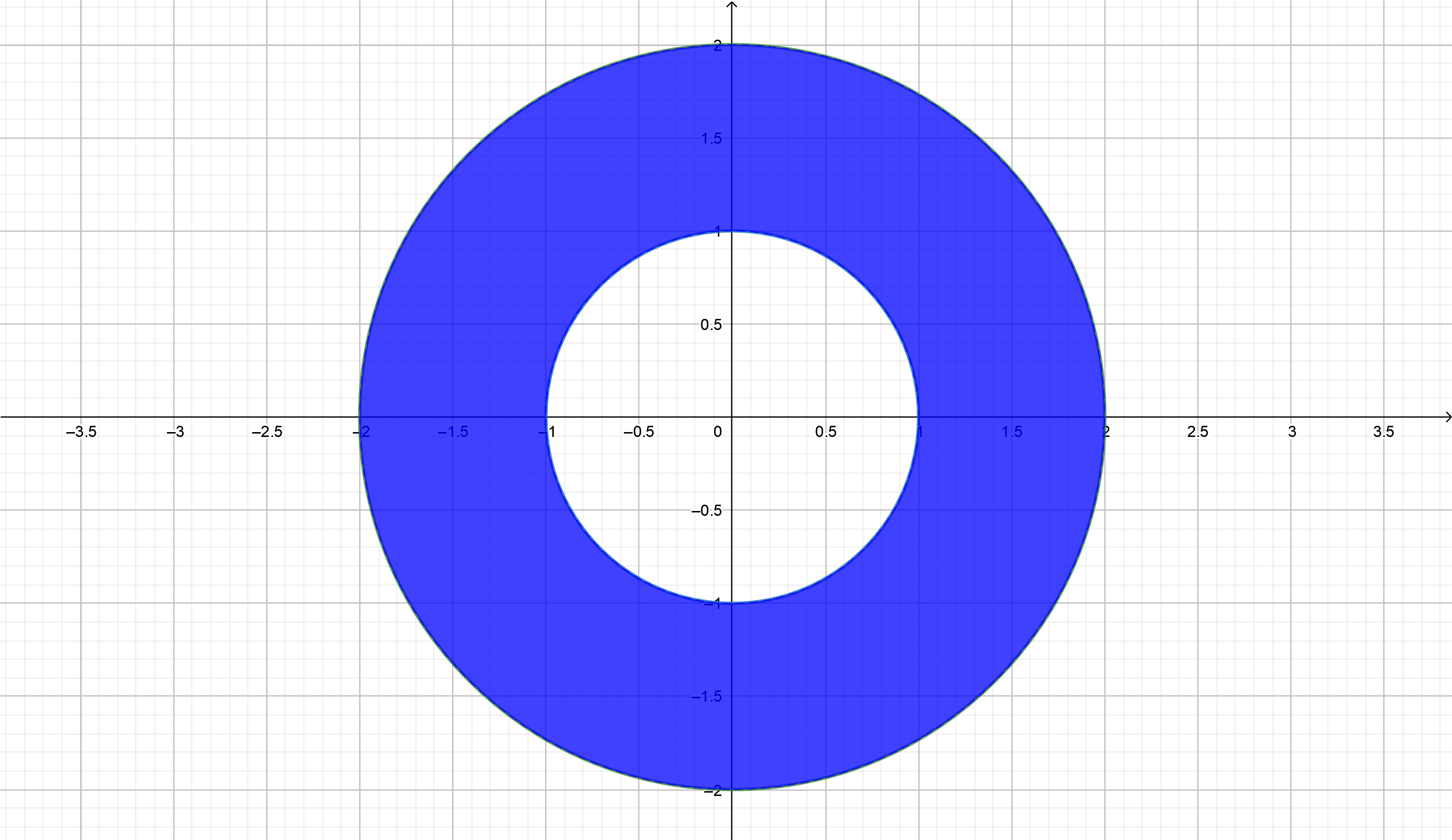
The rectangular equation of the annulus between the circles of radius one and radius two centered at the origin is given by

$$ 1 \le x^2 + y^2 \le 4 $$
and the polar equation of this annulus is given by

$$ 1 \le r \le 2 $$

Example 4

Annular Sector

Rectangular Coordinates	Polar Coordinates

Figure 2

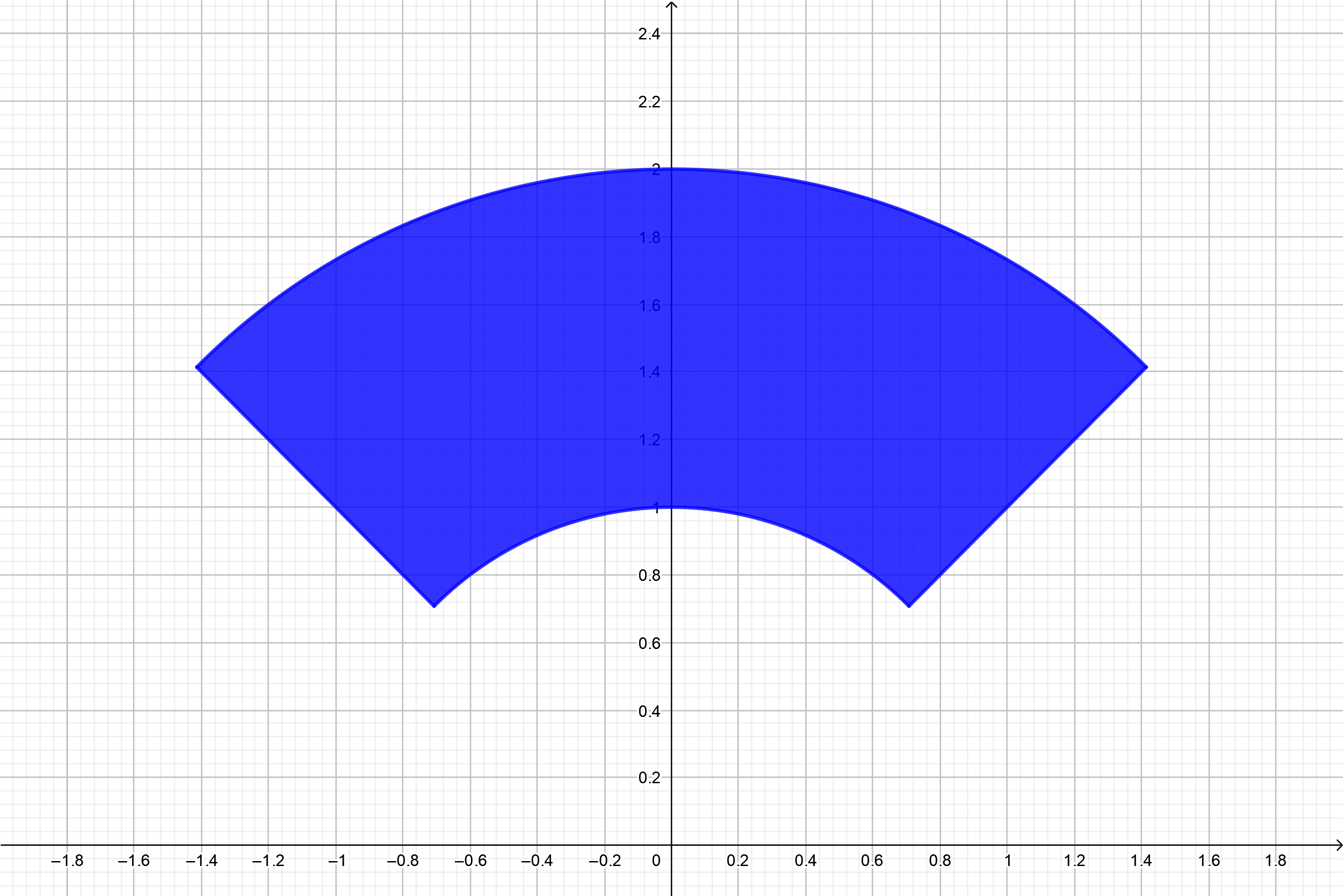
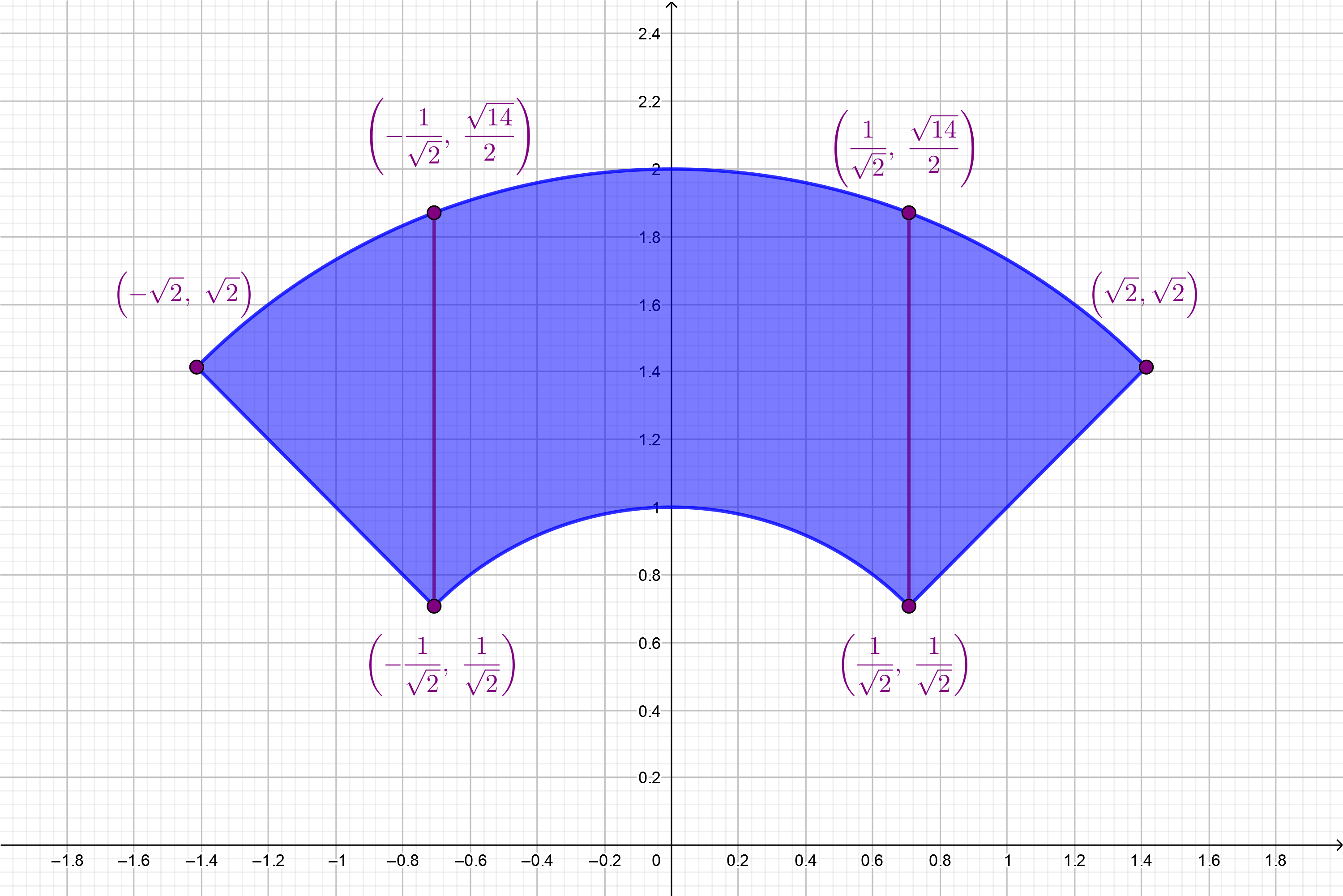
In order to describe an annular sector in rectangular coordinates one must first divide up the region into sub-regions with rectangular edges for at least one variable. This makes describing the annular sector in terms of rectangular coordinate $x$ messy, and adds complicated end points for the intervals of the domain of the piece-wise defined function of $y$ in terms of $x$ over the intervals $\left(-\sqrt{2},\ -\frac{1}{\sqrt{2}}\right)$, $\left(-\frac{1}{\sqrt{2}}, \frac{1}{\sqrt{2}}\right)$, and $\left(\frac{1}{\sqrt{2}},\ \sqrt{2}\right)$.

In polar form the region is represented as a polar rectangle

$$ 1 \le r \le 2,\ \dfrac{\pi}{4} \le \theta \le \dfrac{3\pi}{4}\qquad\text{or}\qquad [1,2]\times\left[\frac{\pi}{4},\ \frac{3\pi}{4}\right] $$

15.3.2 Areas of Polar Rectangles

The area of rectangle in the rectangular coordinate system is straight-forward

$$ \begin{align*} \text{Area} &= \text{base}\ \times\ \text{height} \\ \\ \text{Area} &= \Delta x\Delta y \end{align*} $$

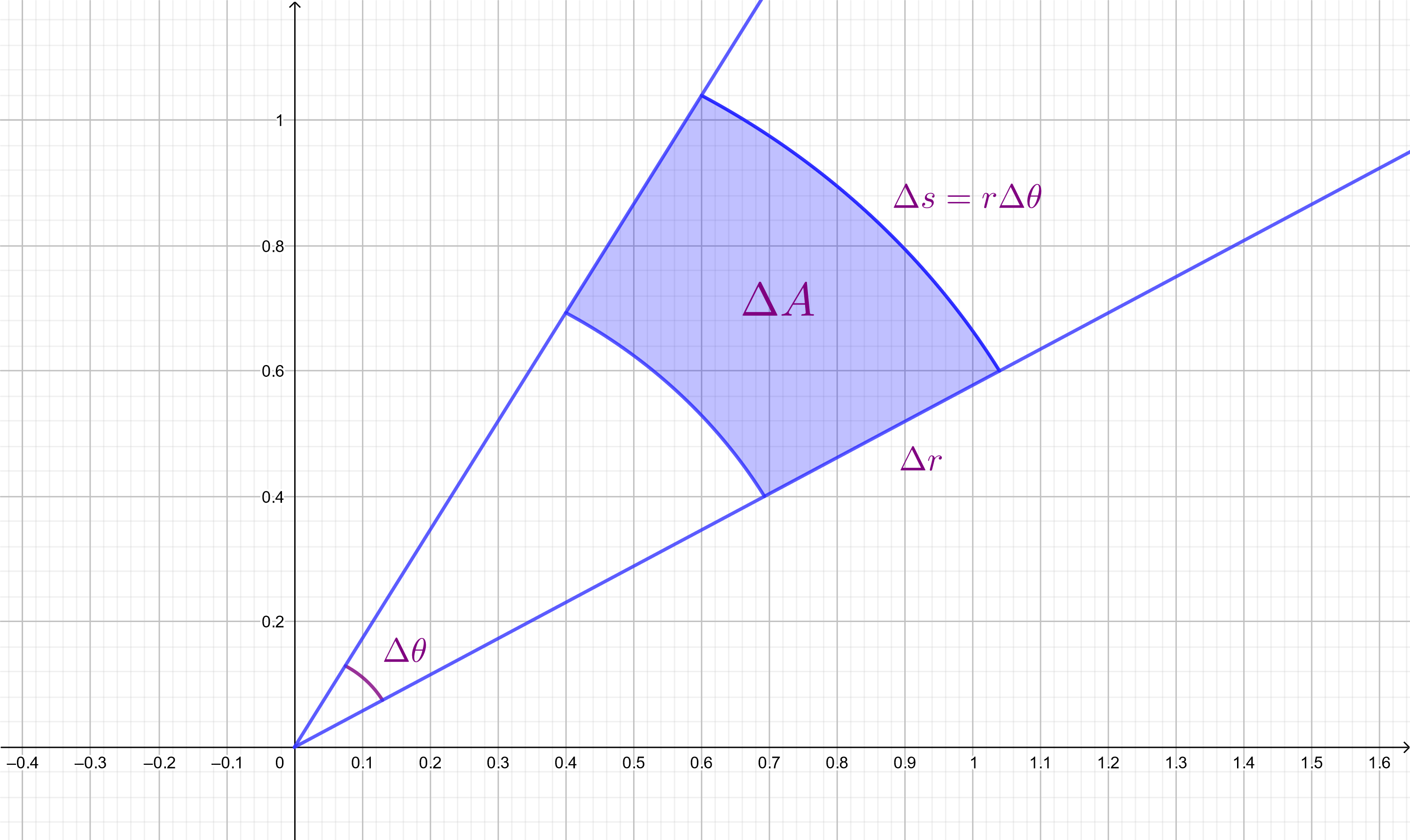
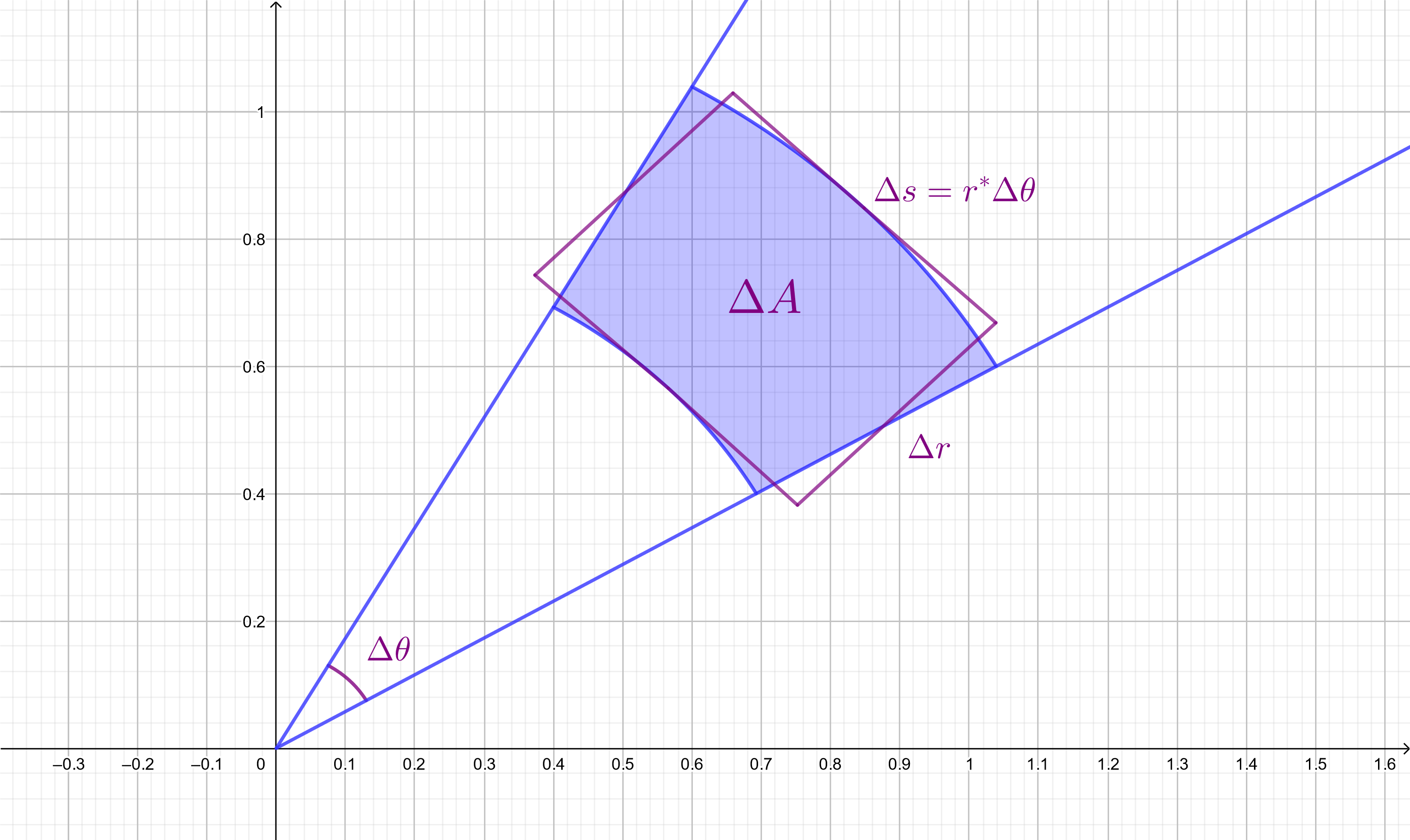
For the polar rectangle, the equation for area is complicated. Instead we approximate the area of the polar rectangle $\left[r_1, r_2\right]\times\left[\theta_1, \theta_2\right]$ with the area of a rectangle with sides $\Delta s$ and $\Delta r = r_2 - r_1$. The height of our rectangle is $\Delta r$ and the width of our rectangle is the arc length of the polar rectangle $\Delta s = s_2 - s_1$. Arc length is a function of the change in angle of the arc $\Delta\theta$ and the radius $r$. Recall the equation for arc length is given by

$$ s = r\theta $$
In order to compute $\Delta s$ we consider that the when $\Delta r$ is small there will not be much difference between any radius $r^{*}\in\left[r_1,r_2\right]$. We define

$$ \Delta s = r^{*}\Delta\theta $$
Thus the area of our polar rectangle is approximated by the area of a rectangle

$$ \Delta A \approx r^{*}\Delta\theta\Delta r = r^{*}\Delta r\Delta\theta $$

One may partition the $xy$-plane into polar rectangles. A set in the $xy$-plane can similarly be approximated by the polar rectangles within the set. As the size of the polar rectangles get smaller, the approximation gets better. The size of a partition is the number of polar rectangles within the set $R$. Smaller polar rectangles means a finer (larger) partition.

There are $M\times N$ polar rectangles in the partition because for each of the $N$ radii $r_k$, the annulus $[r_{k-1}, r_k]\times[0, 2\pi]$ gets partitioned into $M$ polar rectangles


$$ R_{j,k} = [r_{k-1}, r_k]\times[\theta_{j-1}, \theta_j]\qquad 1\le j\le M,\ 1\le k\le N $$
Each polar rectangle has an approximate area

$$ \Delta A_{j,k} \approx r_j^*\Delta r_j\Delta\theta_k $$

Notice from the video and the formula that the size of each polar rectangle in the partition depends on its distance from the origin. This is very different from rectangular coordinates where the size of each rectangle in a partition is the same everywhere on the plane. Rectangular coordinates are translation invariant ; that is, the size of all of the rectangles in the partition of the plane are the same. The area of a polar rectangle always includes its distance from the origin $r_j^*$.

Notice also that the area of a polar rectangle depends only on its radial distance from the origin. Each polar rectangle in a polar annulus will have the same area if the angular interval $[0, 2\pi]$ is partitioned by equally spaced points.

15.3.3 Rectangular Polar Volumes

This differential volume of a rectangular polar solid is given by

Differential Volume = Area of polar rectangle $\ \cdot\ $ height

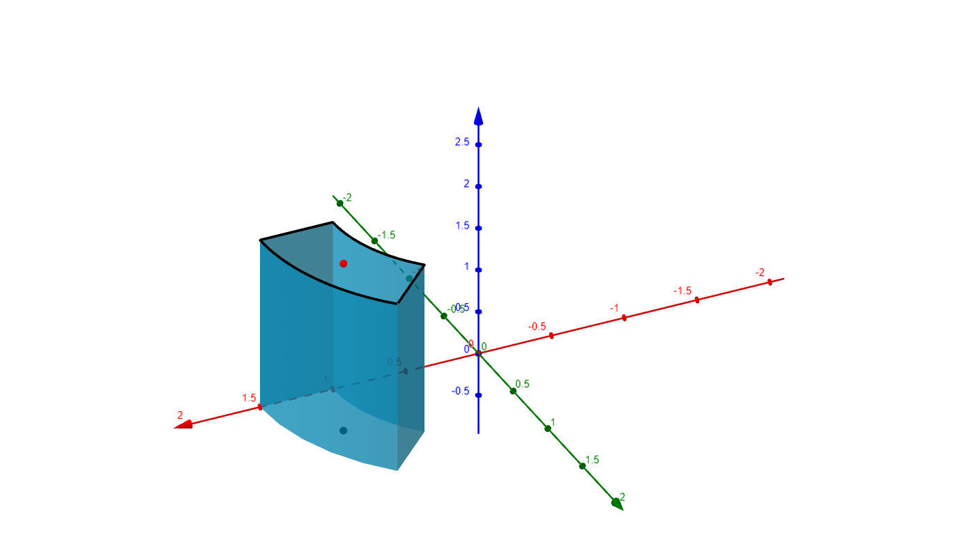
This leads to computing the volume under a surface $\ f(x,y)\ :\ \mathbb{R}^2\rightarrow\mathbb{R}$. For example, given the surface

$$ z = 6 - \dfrac{3x^2}{4} - \dfrac{3y^2}{4}, $$
one may partition the $xy$-plane into polar rectangles, select a point $\left(x^*,y^*\right) = \left(r^*, \theta^*\right)$ in each polar rectangle, and evaluate function $f$ at each point to get a height $f(r^*,\theta^*)$ of the corresponding rectangular polar solid. This results in volume

$$ \begin{align*} V_{j,k} &= \text{height}\,\cdot\,\text{Area }\left(R_{j,k}\right) \\ \\ &= f\left(r_k^*,\theta_j^*\right)\Delta A_{j,k} \\ \\ &= f\left(r_k^*,\theta_j^*\right)r_k^*\Delta r_k\Delta\theta_j \end{align*} $$
If one chooses the point at the outer corner of the polar rectangle each time, video below portrays
1.the polar partition of the $xy$-plane and the images of the polar axes for polar rectangles within the domain of a surface.

1. the first few outer rectangular polar solids form a Riemann sum
2. the first few rows of rectangular polar solids form a Riemann sum

15.3.4 Riemann Sums

If we add up all of the rectangular polar volumes, we obtain a Riemann Sum


$$ S = \displaystyle\sum_{j=1}^M\displaystyle\sum_{k=1}^N V_{j,k} = \displaystyle\sum_{j=1}^M\displaystyle\sum_{k=1}^N f(r_k^*, \theta_j^*)A_{j,k} = \displaystyle\sum_{j=1}^M\displaystyle\sum_{k=1}^N f(r_k^*, \theta_j^*)r_k^*\Delta r_k\Delta\theta_j, $$
where $M\times N$ is the number of polar rectangles in the partition. The limit of the Riemann sums yields

$$ \begin{align*} \displaystyle\iint_R f(r,\theta)\,dA &= \displaystyle\lim_{M,N\rightarrow\infty} \displaystyle\sum_{j=1}^M\displaystyle\sum_{k=1}^N f(r_k^*, \theta_j^*)r_k^*\Delta A_{j,k} \\ \\ &= \displaystyle\lim_{M,N\rightarrow\infty} \displaystyle\sum_{j=1}^M\displaystyle\sum_{k=1}^N f(r_k^*, \theta_j^*)r_k^*\Delta r_k\Delta\theta_j \\ \\ &= \textcolor{brightblue}{\displaystyle\iint_R f(r,\theta)\,r\,dr\,d\theta} \end{align*} $$
Recall that the the double integral in rectangular coordinates is written

$$ \displaystyle\iint_R f(x,y)\,dA = \displaystyle\iint_R f(x,y)\,dx\,dy $$
Thus we have

$$ \displaystyle\iint_R f(x,y)\,dx\,dy = \displaystyle\iint_R f(x,y)\,dA = \displaystyle\iint_R f(r,\theta)\,dA = \textcolor{brightblue}{\displaystyle\iint_R f(r,\theta)\,r\,dr\,d\theta} $$

15.3.5 Fubini's Theorem

Like the formulation of a double integral in rectangular coordinates, the formulation in polar coordinates allow us to use Fubini's Theorem to compute the value of the integral.

Example 5

Compute the volume beneath the surface $z = 4 - x^2 - y^2$ over the circular region of radius 4 centered at the origin.

Thus we must compute

$$ \displaystyle\iint_R \left(4 - x^2 - y^2\right)\,dA $$

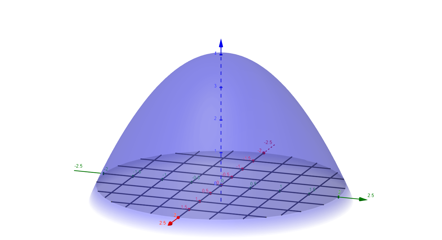
The volume under the paraboloid $z = 4 - x^2 -y^2$, and over the region $x^2 + y^2 \le 4$. In rectangular coordinates we can use the fact that the surface is symmetric with respect to the $z$-axis

$$ \begin{align*} \displaystyle\iint_R \left(4 - x^2 - y^2\right)\,dA &= \displaystyle\iint_R \left(4 - x^2 - y^2\right)\,dy\,dx = 4\displaystyle\int_0^2\displaystyle\int_0^{\sqrt{4-x^2}} \left(4 - x^2 - y^2\right)\,dy\,dx \\ \\ &= 4\displaystyle\int_0^2\left[ 4y - x^2y - \dfrac{y^3}{3} \right]_0^{\sqrt{4-x^2}}\,dx \\ \\ &= 4\displaystyle\int_0^2\left[ 4 - x^2 - \dfrac{4-x^2}{3} \right]\sqrt{4-x^2}\,dx \\ \\ &= \dfrac{8}{3}\displaystyle\int_0^2 \left(4-x^2\right)^{\frac{3}{2}}\,dx\quad\begin{vmatrix} x = 2\sin(\theta) \\ dx = 2\cos(\theta)\,d\theta \end{vmatrix} \\ \\ &= \dfrac{8}{3}\displaystyle\int_0^{\frac{\pi}{2}} \left(4 - 4\sin^2(\theta)\right)^{\frac{3}{2}}2\cos(\theta)\,d\theta \\ \\ &= \dfrac{16}{3}\displaystyle\int_0^{\frac{\pi}{2}}4^{\frac{3}{2}} (1 - \sin^2(\theta))^{\frac{3}{2}}\cos(\theta)\,d\theta \\ \\ &= \dfrac{128}{3}\displaystyle\int_0^{\frac{\pi}{2}} \cos^4(\theta)\,d\theta = \dfrac{128}{3}\displaystyle\int_0^{\frac{\pi}{2}} \left(\cos^2(\theta)\right)^2\,d\theta \\ \\ &= \dfrac{128}{3}\displaystyle\int_0^{\frac{\pi}{2}} \left(\dfrac{1}{2}\left(1 + \cos(2\theta)\right)\right)^2\,d\theta \\ \\ &= \dfrac{32}{3}\displaystyle\int_0^{\frac{\pi}{2}} \left(1 + 2\cos(2\theta) + \cos^2(2\theta)\right)\,d\theta \\ \\ &= \dfrac{32}{3}\displaystyle\int_0^{\frac{\pi}{2}} \left(1 + 2\cos(2\theta) + \dfrac{1}{2}\left(1 + \cos(4\theta) \right)\right)\,d\theta \\ \\ &= \dfrac{16}{3}\displaystyle\int_0^{\frac{\pi}{2}} \left(3 + 4\cos(2\theta) + \cos(4\theta) \right)\,d\theta \\ \\ &= \dfrac{16}{3}\left[3\theta + 2\sin(2\theta) + \dfrac{1}{4}\sin(4\theta) \right]_0^{\frac{\pi}{2}} = \dfrac{16}{3}\cdot\dfrac{3\pi}{2} = 8\pi \\ \end{align*} $$
The computations using polar coordinates use the equation for the surface $z = 4 - r^2$. The disk of radius two $r \le 2$ is a polar rectangle $[0, 2]\times[0, 2\pi]$.

$$ \begin{align*} \displaystyle\iint_R \left(4 - x^2 - y^2\right)\,dA &= \displaystyle\iint_R \left(4 - r^2\right)\,dA \\ \\ &= \displaystyle\iint_R \left(4 - r^2\right)\,r\,dr\,d\theta \\ \\ &= \displaystyle\int_0^{2\pi}\displaystyle\int_0^2 \left(4 - r^2\right)\,r\,dr\,d\theta \\ \\ &= \displaystyle\int_0^{2\pi}\left[ 2r^2 - \dfrac{r^4}{4} \right]_0^2\,d\theta \\ \\ &= \displaystyle\int_0^{2\pi} 8 - 4 \,d\theta = \left[\,4\theta\,\right]_0^{2\pi} = 8\pi\ \color{green}{\Large{\checkmark}} \end{align*} $$
Most will agree the polar coordinates version of the double integral requires fewer steps and less work than the rectangular coordinates version. When computing the value of a double integral, always utilize a strategy that requires simpler and hopefully fewer steps. Generally, using polar coordinates to integrate over regions that display circular symmetry reduce computations.

15.3.6 Compute Volumes Using Polar Coordinates

Exercise 1

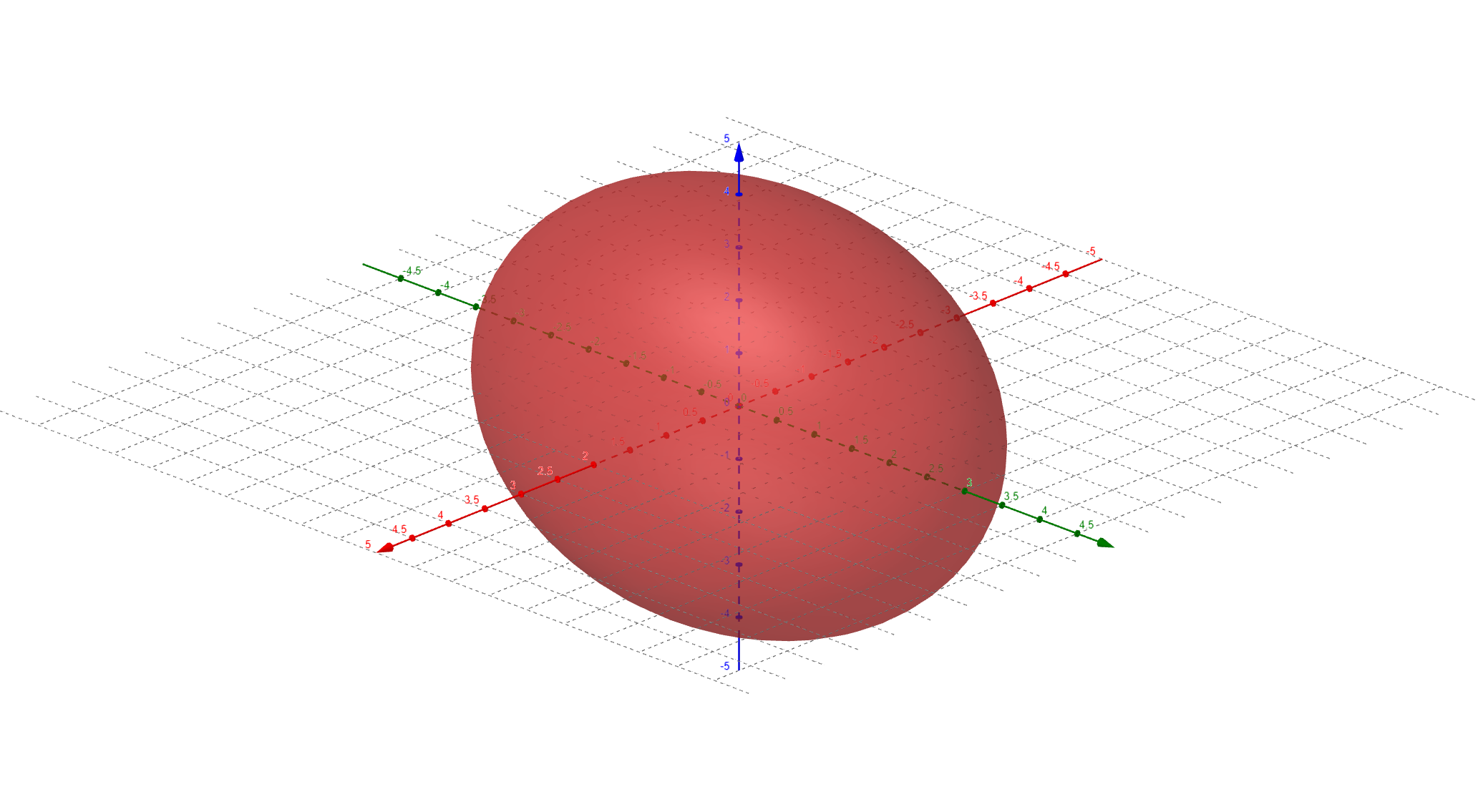
Compute the volume of the ellipsoid

$$ \left(\dfrac{x}{a}\right)^2 + \left(\dfrac{y}{b}\right)^2 + \left(\dfrac{z}{c}\right)^2 = 1 $$

Check your work

Although we can compute the volume using an integral of one variable and compute the volume as a __volume of revolution__, it easier to compute the volume directly using polar coordinates. First consider that the volume is symmetric with respect to the $xy$-plane. So we can compute the total volume by multiplying the volume under the upper surface by two. The upper surface is the surface of the ellipsoid in the upper half-space $z\ge0$. The equation of this surface is given by
$$ z = c\sqrt{1 - \left(\dfrac{x}{a}\right)^2 + \left(\dfrac{y}{b}\right)^2} $$
This gives us Volume $= 2\,\displaystyle\iint_D c\sqrt{1 - \left(\dfrac{x}{a}\right)^2 + \left(\dfrac{y}{b}\right)^2}\,dA$
where $D$ is the area enclosed by the ellipse
$$ \left(\dfrac{x}{a}\right)^2 + \left(\dfrac{y}{b}\right)^2 = 1 $$
At this point the integral is still in terms of rectangular coordinates and we should perform two substitutions for our variables $x$ and $y$
$$ \begin{array}{ccc} x = au & \ & y = bv \\ dx = a\,du & \ & dy = b\,dv \end{array} $$
Likewise $dA = dx\,dy = a\,du\,b\,dv = ab\,du\,dv = ab\,dA'$. The integral for our volume
$$ \text{Volume} = 2abc\,\displaystyle\iint_{D'} \sqrt{1 - u^2 - v^2}\,dA' $$
where $D'$ is the unit circle $u^2 + v^2 = 1$. Now we are ready to convert our integral to polar coordinates.
$$ \begin{align*} \text{Volume} &= 2abc\,\displaystyle\int_0^{2\pi}\displaystyle\int_0^1 \sqrt{ 1 - r^2}\,r\,drd\theta \\ \\ &= 2abc\,\displaystyle\int_0^{2\pi}\,d\theta\cdot\displaystyle\int_0^1 \sqrt{1-r^2}\,r\,dr \\ \\ &= \left|\begin{array}{c} w = 1 - r^2 \\ dw = -2r\,dr \end{array}\right. \\ &= 2abc\ \Big[\,\theta\,\Big]_0^{2\pi}\cdot\displaystyle\int_1^0 \sqrt{w}\,\left(-\dfrac{1}{2}\right)dw \\ \\ &= abc\,\left(2\pi - 0\right)\cdot\left[\,\dfrac{2}{3}w^{3/2}\,\right]_0^1 \\ \\ &= 2\pi\,abc\cdot\dfrac{2}{3} = \dfrac{4}{3}\pi\,abc \end{align*} $$

15.3.7 The Jacobian

Recall the two dimensional iterated integral using polar and rectangular coordinates

$$ \begin{align*} \displaystyle\iint_R f(r,\theta)\,dA &= \displaystyle\iint_R f(r,\theta)\,\textcolor{BrickRed}{r}\,d\theta\,dr = \displaystyle\iint_R f(r,\theta)\,\textcolor{BrickRed}{r}\,dr\,d\theta \\ \\ &= \displaystyle\iint_R f(x(r,\theta), y(r,\theta))\,\textcolor{BrickRed}{r}\,dr\,d\theta \\ \\ &= \displaystyle\iint_R f(x,y)\,dA \\ \\ &= \displaystyle\iint_R f(x,y)\,dx\,dy = \displaystyle\iint_R f(x,y)\,dy\,dx \\ \\ &= \displaystyle\iint_R f(x,y)\textcolor{BrickRed}{\cdot1}\,dx\,dy \end{align*} $$
That is our differential element (or small change ) in area is given by

$$ dA = \textcolor{BrickRed}{r}\,dr\,d\theta = \textcolor{BrickRed}{1}\,dx\,dy $$
The factor , $\textcolor{BrickRed}{r}$ in the case of polar coordinates, and $\textcolor{BrickRed}{1}$ in the case of rectangular coordinates is called the Jacobian . The Jacobian arises because the coordinate system used in the domain determine how small changes in area $\Delta A$ are computed using small changes in the coordinates

• $\Delta A = \Delta x\cdot\Delta y\ $ in rectangular coordinates
• $\Delta A \approx r\,\Delta\theta\cdot\Delta r\ $ in polar coordinates

Everyone should be asking:

1. How does this approximation model we created yield the correct answer when integrating over a circular domain in polar coordinates?
2. How do we use other changes of coordinates (aka substitution) to simplify our computations for non-circular domains?
3. If we use similar geometric intuition to approximate small changes in area for other changes of coordinates, how will we know that the approximation yields the correct answer?

15.3.8 Changes of Coordinates

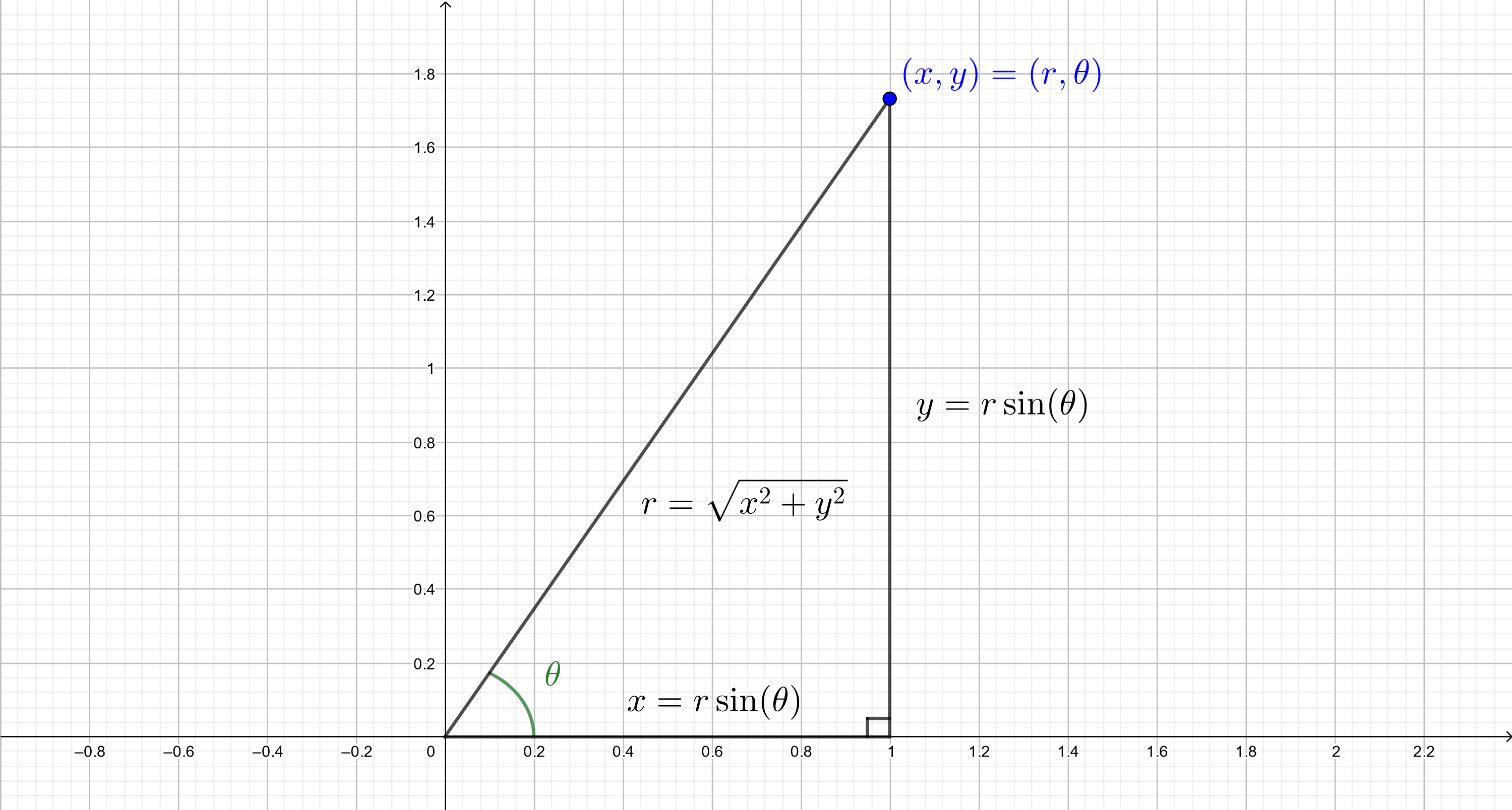
The change of coordinates from rectangular coordinates to polar coordinates are modeled by the following equations

$$ \begin{align*} x &= r\cos(\theta) \qquad &y &= r\sin(\theta) \end{align*} $$
Every point $(x,y)$ on the plane has an associated right triangle with sides of length $x$ and $y$. The coordinate $x$ is the distance left or right along the horizontal axis, and the coordinate $y$ is the distance up or down parallel to the vertical axis. The radial distance $r$ from the origin to the point $(x,y)$ is the length of the hypotenuse of this triangle, and $\theta$ is the angle the hypotenuse or radius makes with the positive $x$-axis.

Now let us use what we know of the differential from chapter 14

$$ \begin{align*} dx &= \dfrac{\partial f}{\partial r}dr + \dfrac{\partial f}{\partial\theta}d\theta \\ \\ &= \dfrac{\partial}{\partial r}\left(r\cos(\theta)\right)dr + \dfrac{\partial}{\partial \theta}\left(r\cos(\theta)\right)d\theta \\ \\ dx &= \cos(\theta)dr - r\sin(\theta)d\theta \\ \\ dy &= \dfrac{\partial}{\partial r}\left(r\sin(\theta)\right)dr + \dfrac{\partial}{\partial \theta}\left(r\sin(\theta)\right)d\theta \\ \\ &= \sin(\theta)dr + r\cos(\theta)d\theta \\ \end{align*} $$
This almost looks like a linear system of equations

$$ \begin{align*} \cos(\theta)dr - r\sin(\theta)d\theta &= dx \\ \sin(\theta)dr + r\cos(\theta)d\theta &= dy \\ \\ \begin{bmatrix} \cos(\theta) & -r\sin(\theta) \\ \sin(\theta) & r\cos(\theta) \end{bmatrix}\,\begin{bmatrix} dr \\ d\theta \end{bmatrix} &= \begin{bmatrix} dx \\ dy \end{bmatrix} \\ \\ \begin{bmatrix} \cos(\theta) & -r\sin(\theta) \\ \sin(\theta) & r\cos(\theta) \end{bmatrix}\,\begin{bmatrix} \Delta r \\ \Delta\theta \end{bmatrix} &= \begin{bmatrix} \Delta x \\ \Delta y \end{bmatrix} \\ \end{align*} $$
We are not yet used to seeing variables in our matrices. However, if we pick a value for the point $(x,y)$, or $(r,\theta)$, so that $r$ and $\theta$ are constants we will have a matrix equation for $\begin{bmatrix} \Delta x \\ \Delta y \end{bmatrix}$ as a function of $\begin{bmatrix} \Delta r \\ \Delta\theta \end{bmatrix}$.

For example if we choose $r = 2$ and $\theta = \dfrac{\pi}{3}$, then

$$ \begin{align*} x = 2\cos\left(\dfrac{\pi}{3}\right) = 2\cdot\frac{1}{2} = 1 \\ \\ y = 2\sin\left(\dfrac{\pi}{3}\right) = 2\cdot\frac{\sqrt{3}}{2} = \sqrt{3} \\ \end{align*} $$
Moreover we have that the linear system of equations for our small changes is given by

$$ \begin{align*} \begin{bmatrix} \cos\left(\dfrac{\pi}{3}\right) & 2\sin\left(\dfrac{\pi}{3}\right) \\ -\sin\left(\dfrac{\pi}{3}\right) & 2\cos\left(\dfrac{\pi}{3}\right) \end{bmatrix}\begin{bmatrix} \Delta r \\ \Delta\theta \end{bmatrix} &= \begin{bmatrix} \Delta x \\ \Delta y \end{bmatrix} \\ \\ \begin{bmatrix} \dfrac{1}{2} & \sqrt{3} \\ -\dfrac{\sqrt{3}}{2} & 1 \end{bmatrix}\begin{bmatrix} \Delta r \\ \Delta\theta \end{bmatrix} &= \begin{bmatrix} \Delta x \\ \Delta y \end{bmatrix} \\\end{align*} $$
This gives us a linear transformation $S = \begin{bmatrix} \dfrac{1}{2} & \sqrt{3} \\ -\dfrac{\sqrt{3}}{2} & 1 \end{bmatrix}$ from the small changes in polar coordinates to the small changes in rectangular coordinates at the point $\begin{bmatrix} 1 \\ \sqrt{3} \end{bmatrix}$.

At this point we need to review the determinant of a matrix and understand the meaning of determinant. There is a fantastic video by Grant Sanderson, The Determinant .

Now that we know that the determinant of a matrix is actually the scaling factor for areas (volumes) of the coordinates, we see our linear system in a new light.

$$ S\begin{bmatrix} dr \\ d\theta \end{bmatrix} = \begin{bmatrix} \dfrac{1}{2} & \sqrt{3} \\ -\dfrac{\sqrt{3}}{2} & 1 \end{bmatrix}\begin{bmatrix} dr \\ d\theta \end{bmatrix} = \begin{bmatrix} dx \\ dy \end{bmatrix} $$
not only gives us a way of mapping small changes in polar coordinates to rectangular coordinates; it also give us the scaling factor for mapping areas $\Delta A' = dr\,d\theta$ to $\Delta A = dx\,dy$ at the point $\begin{bmatrix} 1 \\ \sqrt{3} \end{bmatrix}$. This scaling factor is

$$ \text{abs}\left(\text{det}(A)\right) = \left|\text{det}(A)\right| $$
Determinants may be negative indicating a change in the orientation of the coordinates, however areas are always non-negative so we will use the absolute value of the determinant. The scaling factor is

$$ \begin{align*} \left|\text{det}(A)\right| &= \left|\,\text{det} \begin{bmatrix} \dfrac{1}{2} & \sqrt{3} \\ -\dfrac{\sqrt{3}}{2} & 1 \end{bmatrix} \,\right| \\ \\ &= \left| \dfrac{1}{2} - \left(-\frac{3}{2}\right) \right| = 2 \\ \end{align*} $$
This tells us that small changes in area at the point $\begin{bmatrix} 1 \\ \sqrt{3} \end{bmatrix}$ is given by

$$ \left|\text{det}(S)\right|\Delta A' = 2\Delta r\,\Delta\theta = \Delta x\,\Delta y = \Delta A, $$
or in differentials

$$ \left|\text{det}(S)\right|dA' = 2dr\,d\theta = dx\,dy = dA. $$
Furthermore we have a matrix-valued function

$$ S = S(r,\theta) = \begin{bmatrix} \cos(\theta) & -r\sin(\theta) \\ \sin(\theta) & r\cos(\theta) \end{bmatrix} $$
This yields the transition matrix for our small changes in area at every point on the plane. We may compute the determinant of $S(r,\theta)$ to determine a formula for the scaling factor (Jacobian) for every point.

$$ \begin{align*} \left|\text{det}\left(S(r,\theta)\right)\right| &= \text{abs}\left(\text{det}\left(\begin{bmatrix} \cos(\theta) & -r\sin(\theta) \\ \sin(\theta) & r\cos(\theta) \end{bmatrix} \right)\right) \\ \\ &= \left| r\cos^2(\theta) + r\sin^2(\theta) \right| = r. \end{align*} $$
We don't need absolute value signs for the radial distance $r$ because $r\ge 0$. These computations give us the Jacobian as the scaling factor for the linear transformation $S$ from small changes in polar coordinates to small changes in rectangular coordinates. Thus

$$ r\,dA' = r\,dr\,d\theta = dx\,dy = dA $$

15.3.9 Exercises

Exercise 2

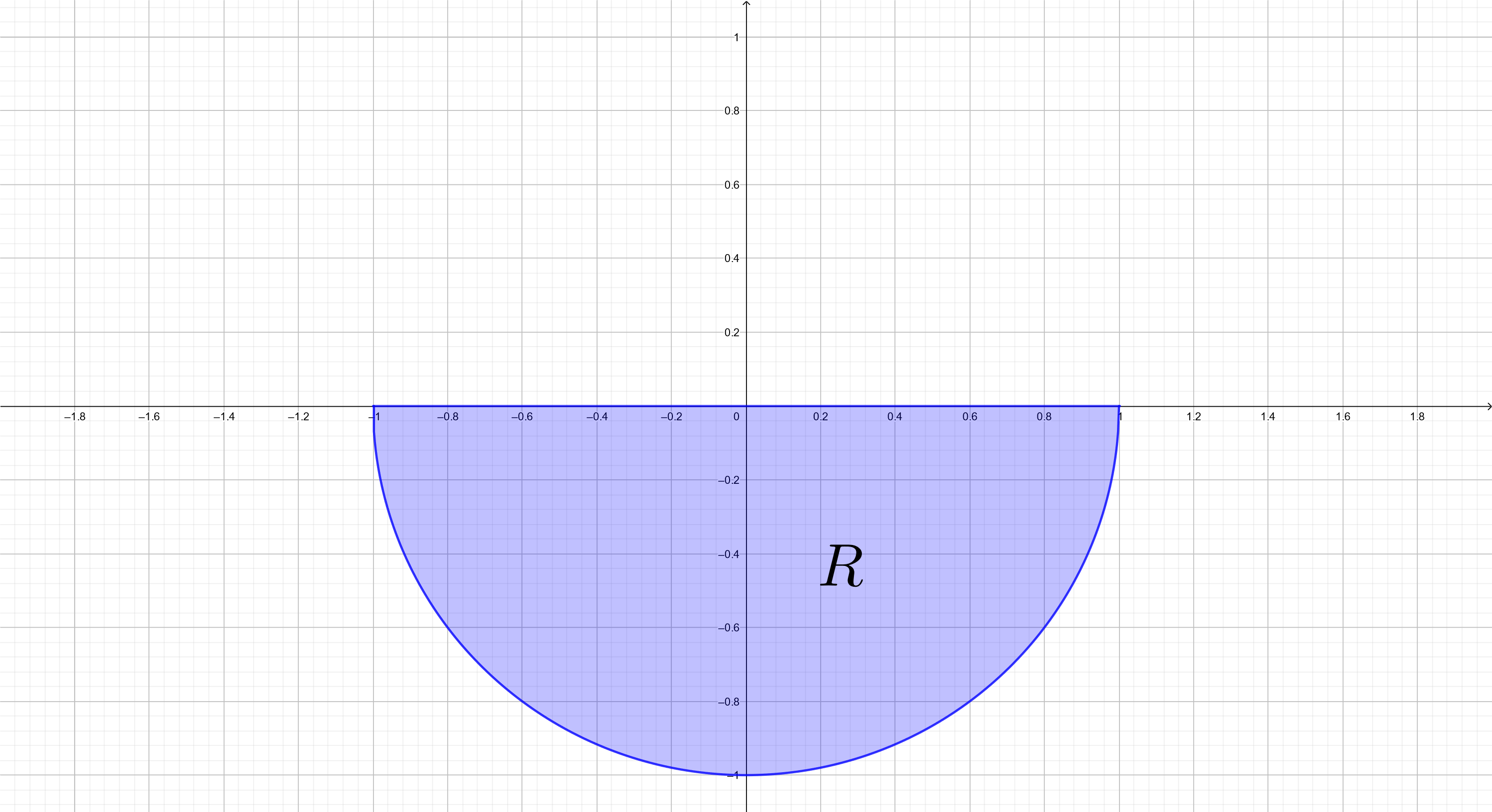
Consider the function $f(x,y) = 3x^2 + y^2$. Find the volume under the surface $z = f(x,y)$ over the region $R$.

Check your work

Computing an iterated integral yields


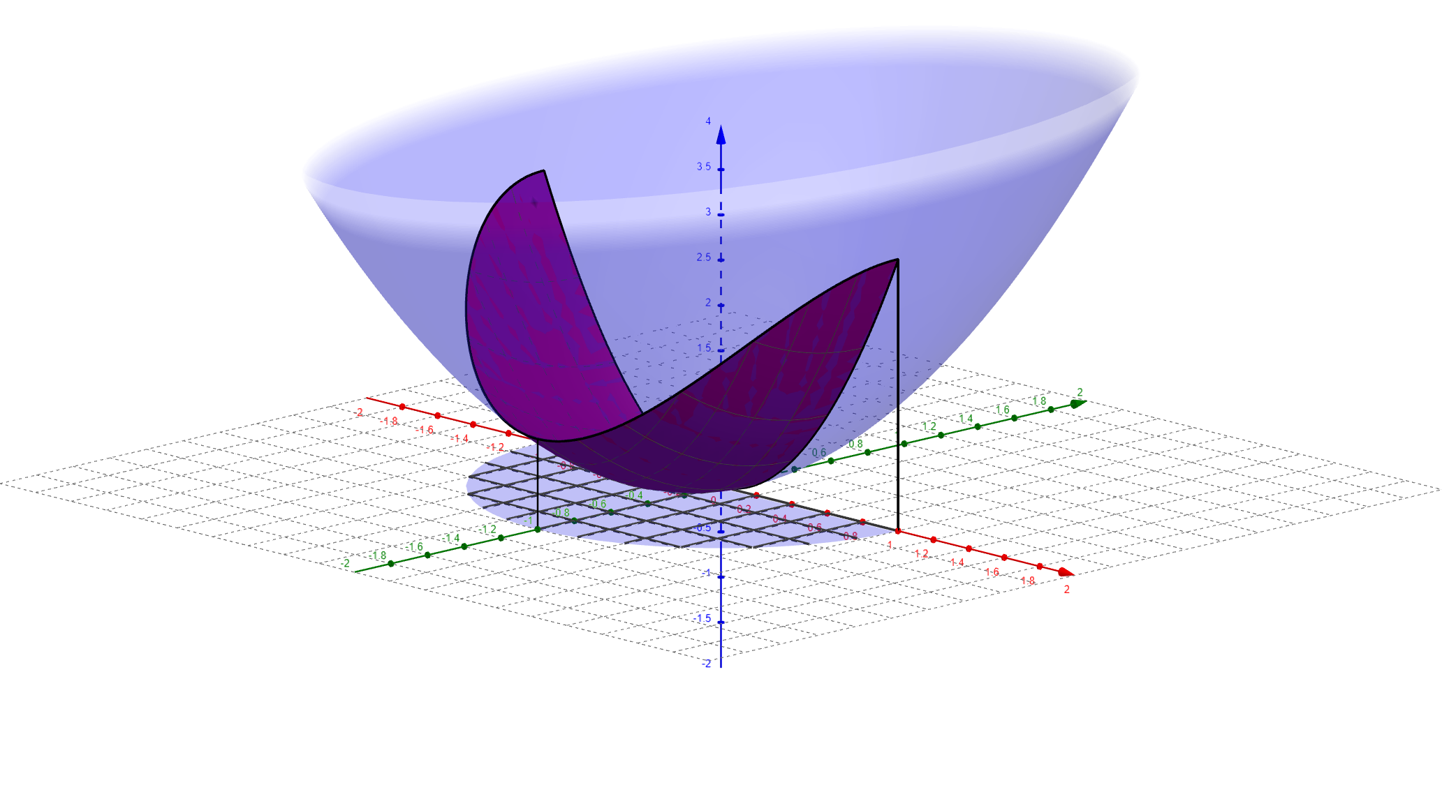
$$ \begin{align*} \text{Volume} &= \displaystyle\iint_R 3x^2 + y^2\,dA \\ \\ &= \displaystyle\iint_R 2x^2 + x^2 + y^2\,dA \\ \\ &= \displaystyle\int_{\pi}^{2\pi}\displaystyle\int_0^1\left(2r^2\cos^2(\theta) + r^2\right)\,r\,dr\,d\theta \\ \\ &= \displaystyle\int_{\pi}^{2\pi}\displaystyle\int_0^1\left(2\cos^2(\theta) + 1\right)\,r^3\,dr\,d\theta \\ \\ &= \displaystyle\int_{\pi}^{2\pi}\displaystyle\int_0^1\left(2\cos^2(\theta) - 1 + 2\right)\,r^3\,dr\,d\theta \\ \\ &= \displaystyle\int_{\pi}^{2\pi}\cos(2\theta) + 2\,d\theta\cdot \displaystyle\int_0^1r^3\,dr \\ \\ &= \left[ \dfrac{1}{2}\sin(2\theta) + 2\theta\right]_{\pi}^{2\pi} \cdot \left[ \dfrac{r^3}{3}\right]_0^1 \\ \\ &= \left[ 0 + 4\pi - \left( 0 + 2\pi \right) \right]\cdot\left[\dfrac{1}{3} - 0\right] = \dfrac{2\pi}{3} \\ \end{align*} $$

Your use of this self-initiated mediated course material is subject to our Creative Commons License .

Creative Commons Attribution-NonCommercial-ShareAlike 4.0


Attribution
You must give appropriate credit, provide a link to the license, and indicate if changes were made. You may do so in any reasonable manner, but not in any way that suggests the licensor endorses you or your use.


Noncommercial
You may not use the material for commercial purposes.


Share Alike
You are free to share, copy and redistribute the material in any medium or format. If you adapt, remix, transform, or build upon the material, you must distribute your contributions under the same license as the original.