1.3 Applications 
 1.3 Applications
 Each Section and Topic title are links. At the end of each section, there is a link back to this table.
- 1.3.1 Partial Fraction Decomposition
- 1.3.2 Stoichiometry
- 1.3.3 Exercises
- Exercise 1 - Systems of Linear Equations
- Definition: Transition of Probabilities Matrices
- Exercise 2 - Transition of Probabilities Matrices
- Figure 1: A Transition Probabilities Graph
- Table 1: Transition Probabilities by Parent
- Exercise 3 - Network Analysis
- Figure 2: A Network Flow Graph
- Exercise 4 - Circuit Analysis
- Figure 3: An Electrical Circuit
- Figure 4: The Circuit with Loop Paths
- 1.3.4 Short Answer Exercises
- 1.3.5 True/False Questions
- 1.3.6 Multiple Choice Questions
- 1.3.7 Challenge Exercises
- copyleft
1.3.1 Partial Fraction Decomposition
Systems of Linear Equations occur in many applications, including applications that do not appear to be linear.
Example 1 - Partial Fraction Decomposition
Compute the integral
$$ \int\dfrac{x^2 + 4x + 1}{x^3 - x^2 - x + 1}\,dx $$
The easiest method of integrating this function utilizes a method called partial fraction decomposition. First one must factor the denominator. The Rational Root Theorem states that any rational root of $x^3-x^2-x+1$ must be a ratio whose numerator is a factor of the leading coefficient $1$, and whose denominator is a factor of the constant term $1$. So all rational roots will be
$$ r = \pm 1 $$
We can try the root $1$ by dividing the polynomial by $x-1$ using synthetic division
$$ \begin{array}{cccccc} 1 & | & 1 & -1 & -1 &\ \ 1 \\ & & &\ \ 1 &\ \ 0 & -1 \\ \hline & & 1 &\ \ 0 & -1 &\ \ 0 \\ \end{array} $$
So
$$ x^3 - x^2 - x + 1 = (x-1)(x^2 - 1) = (x-1)(x-1)(x+1) = (x-1)^2(x+1) $$
This means we can re-write our rational integrand
$$ \begin{align*} \dfrac{x^2 + 4x + 1}{x^3 - x^2 - x + 1} &= \dfrac{A}{x-1} + \dfrac{B}{(x - 1)^2} + \dfrac{C}{x+1} \\ \\ &= \dfrac{A(x-1)(x+1)}{(x-1)^2(x+1)} + \dfrac{B(x+1)}{(x-1)^2(x+1)} + \dfrac{C(x-1)^2}{(x-1)^2(x+1)} \\ \\ &= \dfrac{A(x^2-1) + B(x+1) + C(x^2 - 2x + 1)}{(x-1)^2(x+1)} \end{align*} $$
Ignoring our denominators yields
$$ \begin{align*} x^2 + 4x + 1 &= A(x^2-1) + B(x+1) + C(x^2 - 2x + 1) \\ \\ &= Ax^2 - A + Bx + B + Cx^2 - 2Cx + C \\ \\ &= (A + C)x^2 + (B - 2C)x + (-A + B + C) \end{align*} $$
In order for these two quadratic polynomials to be equal we must have
$$ \begin{align*} A \ \ \ \ \ \ \ \ \ \ +\ \ C &= 1 \\ \ \ \ \ \ B - 2C &= 4 \\ -A\ + \ B +\ \ C &= 1 \end{align*} $$
This is a linear system. In order to solve this linear system, or complete this integration we perform Gaussian Elimination.
$$ \begin{align*} \left[ \begin{array}{ccc|c}\ \ 1\ &\ \ 0\ &\ \ 1\ &\ \ 1\ \\ \ \ 0\ &\ \ 1\ & -2\ &\ \ 4\ \\ -1\ &\ \ 1\ &\ \ 1\ &\ \ 1\ \end{array} \right] \begin{array}{l} \\ \\ R_3+R_1 \end{array} &\longrightarrow \left[ \begin{array}{ccc|c}\ \ 1\ &\ \ 0\ &\ \ 1\ & | &\ \ 1\ \\ \ \ 0\ &\ \ 1\ & -2\ & | &\ \ 4\ \\ \ 0\ &\ \ 1\ &\ \ 2\ & | &\ \ 2\ \end{array} \right] \begin{array}{l} \\ \\ R_3-R_2 \end{array} \longrightarrow \\ \\ \left[ \begin{array}{ccc|c}\ \ 1\ &\ \ 0\ &\ \ 1\ &\ \ 1\ \\ \ \ 0\ &\ \ 1\ & -2\ &\ \ 4\ \\ \ 0\ &\ \ 0\ &\ \ 4\ & -2\ \end{array} \right] \begin{array}{l} \\ \\ \frac{1}{4}R_3 \quad\ \ \end{array} &\longrightarrow \left[ \begin{array}{ccc|c}\ \ 1\ &\ \ 0\ &\ \ 1\ & | &\ \ 1\ \\ \ \ 0\ &\ \ 1\ & -2\ & | &\ \ 4\ \\ \ 0\ &\ \ 0\ &\ \ 1\ & | & -\frac{1}{2}\ \end{array} \right] \begin{array}{l} R_1-R_3 \\ R_2+2R_3 \\ \\ \end{array} \longrightarrow \\ \\ \left[ \begin{array}{ccc|c}\ \ 1\ &\ \ 0\ &\ \ 0\ &\ \ \frac{3}{2}\ \\ \ \ 0\ &\ \ 1\ &\ \ 0\ &\ \ 3\ \\ \ 0\ &\ \ 0\ &\ \ 1\ & -\frac{1}{2}\ \end{array} \right] \end{align*} $$
Thus
$$ \dfrac{x^2 + 4x + 1}{x^3 - x^2 - x + 1} = \dfrac{\frac{3}{2}}{x-1} + \dfrac{3}{(x - 1)^2} - \dfrac{\frac{1}{2}}{x+1} $$
Each of these terms is easier to integrate.
$$ \begin{align*} f(x) &= \displaystyle\int \dfrac{x^2 + 4x + 1}{x^3 - x^2 - x + 1}\,dx \\ \\ &= \displaystyle\int \left(\dfrac{\frac{3}{2}}{x-1} + \dfrac{3}{(x - 1)^2} - \dfrac{\frac{1}{2}}{x+1}\right)\,dx \\ \\ &= \frac{3}{2}\displaystyle\int \dfrac{1}{x-1}\,dx + 3\displaystyle\int \dfrac{1}{(x - 1)^2}\,dx - \frac{1}{2}\displaystyle\int \dfrac{1}{x+1}\,dx \\ \\ &= \frac{3}{2}\ln\left|x-1\right| - 3(x-1)^{-1} - \frac{1}{2}\ln\left|x+1\right| + C \\ \\ &= \frac{1}{2}\ln\left(\dfrac{|x-1|^3}{|x+1|}\right) - \dfrac{3}{x-1} + C \end{align*} $$
on the interval $(-1,1)$.
Notice that a problem that appears to be very nonlinear is still solved using a system of linear equations.

1.3.2 Stoichiometry
Example 2 - Balancing a Chemical Reaction Equation
Liquid benzene burns in the atmosphere. If a cold object is placed directly over the benzene, water will condense on the object and a deposit of soot (carbon) will form on the object. The chemical equation for this reaction is
$$ x_1C_6H_6 + x_2O_2 \longrightarrow x_3C + x_4H_2O $$
Determine the values of $x_1$, $x_2$, $x_3$, and $x_4$ to balance the equation.
A system of linear equations emerges from balancing the equation:
$$ \begin{align*} 6x_1C &= x_3C \\ 6x_1H &= 2x_4H \\ 2x_2O &= x_4O \end{align*} $$
This linear system of equation can be re-written
$$ \begin{align*} 6x_1 \quad\quad\quad - x_3\quad\quad\quad &= 0 \\ 6x_1 \,\ \quad\quad\quad\quad\quad -2x_4 &= 0 \\ 2x_2 \quad\quad\quad -x_4 &= 0 \end{align*} $$
This homogeneous linear system is underdetermined. One solves the linear system by reducing the augmented matrix,
$$ \begin{align*} \begin{bmatrix}\ \ 6\ &\ \ 0\ & -1\ &\ \ 0\ \\ \ \ 6\ &\ \ 0\ &\ \ 0\ & -2\ \\ \ \ 0\ &\ \ 2\ &\ \ 0\ & -1\ \end{bmatrix}\begin{array}{l} \\ R_2-R_1 \\ \\ \end{array} &\rightarrow \begin{bmatrix}\ \ 6\ &\ \ 0\ & -1\ &\ \ 0\ \\ \ \ 0\ &\ \ 0\ &\ \ 1\ & -2\ \\ \ \ 0\ &\ \ 2\ &\ \ 0\ & -1\ \end{bmatrix}\begin{array}{l} \\ R_3 \\ R_2 \\ \end{array} \\ \\ &\rightarrow \begin{bmatrix}\ \ 6\ &\ \ 0\ & -1\ &\ \ 0\ \\ \ \ 0\ &\ \ 2\ &\ \ 0\ & -1\ \\ \ \ 0\ &\ \ 0\ &\ \ 1\ & -2\ \end{bmatrix}\begin{array}{l} R_1+R_3 \\ \\ \\ \end{array} \qquad\text{Row Echelon Form} \\ \\ &\rightarrow \begin{bmatrix}\ \ 6\ &\ \ 0\ &\ \ 0\ & -2\ \\ \ \ 0\ &\ \ 2\ &\ \ 0\ & -1\ \\ \ \ 0\ &\ \ 0\ &\ \ 1\ & -2\ \end{bmatrix} \qquad\qquad\qquad\text{Hermite Normal Form} \end{align*} $$
Definition
Hermite Normal Form
The Hermite Normal Form of an $m\times n$ matrix $A$ is a row equivalent matrix in reduced row echelon form save that the pivots are not required to be $1$. Instead the matrix must satisfy
- upper triangular form
- zeros above and below the pivots
- all coefficients in the matrix must be integers, no nontrivial denominators
Hermite normal form is used in cryptography, integer programming, and chemistry. One typically wants integer coefficients for a balanced equation.
Continuing with backward substitution
$$ \begin{align*} x_4 &= s \in\mathbb{R} \\ \\ x_3 - 2s &= 0 \\ x_3 &= 2s \\ \\ 2x_2 - s &= 0 \\ x_2 &= \frac{s}{2} \\ \\ 6x_1 - 2s &= 0 \\ x_1 &= \frac{s}{3} \\ \\ \text{Solution} &= \left\{\, \begin{bmatrix}\ \frac{s}{3}\ \\ \ \frac{s}{2}\ \\ \ 2s\ \\ \ s\ \end{bmatrix} \,\right\} \end{align*} $$
The smallest value of $s$ that gives us a solution with integer coefficients is the least common multiple of the denominators, $s=6$. Hence to balance the equation we use the solution
$$ \mathbf{x} = \begin{bmatrix}\ 2\ \\ \ 3\ \\ 12\ \\ \ 6\ \end{bmatrix} $$
The balanced chemical equation becomes
$$ 2C_6H_6 + 3O_2 \longrightarrow 12C + 6H_2O $$
1.3.3 Exercises
Application Exercises
Exercise 1 - Systems of Linear Equations
Determine the values of $k$ such that the system of linear equations is inconsistent.
$$
\begin{align*}
kx +\ \ y &= 0 \\
x + ky &= 1
\end{align*}
$$
Check Your Work
$k = 1$ and $k = -1$.
Follow Along
We can re-write the order of the equations
$$ \begin{align*} x + ky &= 1 \\ kx +\ \ y &= 0 \end{align*} $$
Case 1: $k=0$
If $k=0$, then we have $x=1$ and $y=0$ and the linear system of equations is consistent because it has a solution.
Now if $k\neq 0$,
$$ \begin{align*} \begin{bmatrix}\ \ 1\ &\ \ k\ & | &\ \ 1\ \\ \ \ k\ &\ \ 1\ & | &\ \ 0\ \end{bmatrix}\begin{array}{l} \\ R_2-kR_1 \end{array} &\rightarrow\begin{bmatrix}\ \ 1\ &\ \ k\ & | &\ \ 1\ \\ \ \ 0\ & 1-k^2 & | & -k\ \end{bmatrix} \end{align*} $$
Case 2: $(1-k^2)\neq 0$
$$ \begin{align*} \begin{bmatrix}\ \ 1\ &\ \ k\ & | &\ \ 1\ \\ \ \ 0\ & 1-k^2 & | & -k\ \end{bmatrix}\begin{array}{l} \\ \frac{1}{1-k^2}R_2 \end{array} &\rightarrow\begin{bmatrix}\ \ 1\ &\ \ k\ & | &\ \ 1\ \\ \ \ 0\ &\ \ 1\ & | & -\frac{k}{1-k^2}\ \end{bmatrix}\begin{array}{l} R_1-kR_2 \\ \\ \end{array} \\ \\ &\rightarrow\begin{bmatrix}\ \ 1\ &\ \ 0\ & | &\ \frac{1}{1-k^2}\ \\ \ \ 0\ &\ \ 1\ & | & -\frac{k}{1-k^2}\ \end{bmatrix} \end{align*} $$
or
$$ \begin{align*} x &=\ \ \frac{1}{1-k^2} \\ y &= -\frac{k}{1-k^2} \end{align*} $$
Thus we have a solution $x=\frac{1}{1-k^2}$ and $y=-\frac{k}{1-k^2}$ so the system of linear equations is still consistent.
Case 3: $(1-k^2) = 0$
However, if $1-k^2=0$, then $k=\pm 1$ we have
$$ \begin{bmatrix}\ \ 1\ & \pm 1\ & | &\ \ 1\ \\ \pm 1\ &\ \ 1\ & | &\ \ 0\ \end{bmatrix} $$
Each of these linear systems is inconsistent.
$$ \begin{align*} \begin{bmatrix}\ \ 1\ &\ \ 1\ & | &\ \ 1\ \\ \ \ 1\ &\ \ 1\ & | &\ \ 0\ \end{bmatrix}\begin{array}{l} \\ R_2-R_1 \end{array} &\rightarrow\begin{bmatrix}\ \ 1\ &\ \ 1\ & | &\ \ 1\ \\ \ \ 0\ &\ \ 0\ & | & -1\ \end{bmatrix} \end{align*} $$
$$ \begin{align*} \begin{bmatrix}\ \ 1\ & -1\ & | &\ \ 1\ \\ -1\ &\ \ 1\ & | &\ \ 0\ \end{bmatrix}\begin{array}{l} \\ R_2+R_1 \end{array} &\rightarrow\begin{bmatrix}\ \ 1\ & -1\ & | &\ \ 1\ \\ \ \ 0\ &\ \ 0\ & | &\ \ 1\ \end{bmatrix} \end{align*} $$
Exercise 2 - Transition of Probabilities Matrices
Definition
Transition of Probabilities Matrices
A stochastic matrix or transition of probabilities matrix is an $m\times n$ matrix $A$ of nonnegative real numbers, such that the sums of each column of entries is equal to one.
That is for each column $\mathbf{a}_j$ of matrix $A$,
$$ \sum_{i=1}^m a_{ij} = 1 $$
Usually all of the entries are probabilities or numbers in the interval $[0,1]$. Each probability $a_{ij}$ represents the probability that a member of a population currently occupying state $j$ will transition to state $i$ in the next time step.
Assume that the children of 80 percent of Harvard graduates also attend Harvard and the rest attend Yale. Consider also that 40 percent of the children of Yale graduates attend Yale, and the rest split evenly between Harvard and Dartmouth. The children of Dartmouth graduates are 70 percent likely to attend Dartmouth, 20 percent attend Harvard, and 10 percent attend Yale.
Draw the directed graph illustrating the change of state probability from one generation of graduates to the next for each University.
Create the Transition Probabilities Matrix $P$ for this directed graph.
The transition probabilities matrix for the grandchildren of University graduates will be $P^2$. Compute $P^2$.
What is the probability that the grandchild of a Harvard graduate attends Harvard?
Check Your Work
1. You must create a directed graph with a circle for each University or state of the linear system. The directed arrows are labeled with the probability that next generation will transition from their father's state to another.
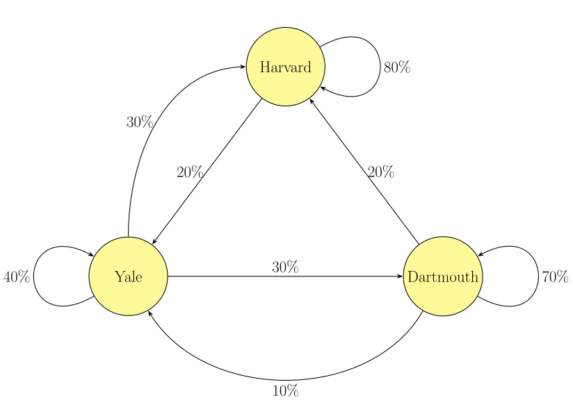
Notice that the sum of the probabilities of the out arrows for each state (or node) equals $100\%$. This indicates that the children of the graduates of these Universities all attend one of them. If some chose not to attend college, we would need a no university state for these children.
2. We can create a table with the transition probabilites for each state. The columns represent the nodes of the directed graph. In other words, the alma mater of one's parent. Each element of the column contains the transition probability from the parent University to the child's.
| Parent | Harvard | Yale | Dartmouth |
|---|---|---|---|
| Harvard | .8 | .2 | 0 |
| Yale | .3 | .4 | .3 |
| Dartmouth | .2 | .1 | .7 |
We can create the transition probabilities matrix from either the graph or the table
$$ P = \begin{bmatrix} .8 & .3 & .2 \\ .2 & .4 & .1 \\ 0 & .3 & .7 \end{bmatrix} $$
3. $P^2 = \begin{bmatrix} .8 & .3 & .2 \\ .2 & .4 & .1 \\ 0 & .3 & .7 \end{bmatrix}\,\begin{bmatrix} .8 & .3 & .2 \\ .2 & .4 & .1 \\ 0 & .3 & .7 \end{bmatrix} = \begin{bmatrix} 0.70 & 0.42 & 0.33 \\ 0.24 & 0.25 & 0.15 \\ 0.06 & 0.33 & 0.52 \end{bmatrix}$
Notice that the sum of each column is still $100\%$ so $P^2$ is also a transition probabilities matrix. It contains the transition probabilites of for each generation's state after two steps.
4. The transition probability for the grandchild of a Harvard graduate attending Harvard is $70\%$ since $(P^2)_{11}$ is the transition probability of a transition from Harvard to Harvard after two generations (steps).
Exercise 3 - Network Analysis
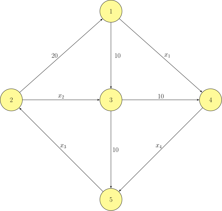
Consider the following network. Assume that the flow into each node into the network is equal to the flow out of each network, FLOW IN = FLOW OUT.
Check Your Work
$\mathbf{x} = \begin{bmatrix}\ 10\ \\ \ 10\ \\ \ 30\ \\ \ 20\ \end{bmatrix}$
Follow Along
From the directed graph we have
$$ \begin{align*} x_1 + 10 &= 20 \\ x_2 + 10 &= 20 \\ x_3 &= x_2 + 20 \\ x_3 &= x_4 + 10 \\ x_4 &= x_1 + 10 \end{align*} $$
From this system of linear equations we can simplify.
$$ \begin{align*} x_1\ \ \ \ \ \ \ \ \ \ \ \ \ \ \ \ \ \ \ \ \ \ \ \ \ \ \ \ &= 10 \\ x_2\ \ \ \ \ \ \ \ \ \ \ \ \ \ \ \ \ \ &= 10 \\ - x_2 + x_3\ \ \ \ \ \ \ \ \ &= 20 \\ x_3 - x_4 &= 10 \\ -x_1\ \ \ \ \ \ \ \ \ \ \ \ \ \ \ \ \ \ + x_4 &= 10 \\ \\ \begin{bmatrix}\ \ 1\ &\ \ 0\ &\ \ 0\ &\ \ 0\ & | & \ 10\ \\ \ \ 0\ &\ \ 1\ &\ \ 0\ &\ \ 0\ \ & | & \ 10\ \\ \ \ 0\ & -1\ &\ \ 1\ &\ \ 0\ \ & | & \ 20\ \\ \ \ 0\ &\ \ 0\ &\ \ 1\ & -1\ \ & | & \ 10\ \\ -1\ &\ \ 0\ &\ \ 0\ &\ \ 1 \ & | & \ 10\ \end{bmatrix}\begin{array}{l} \\ \\ R_3+R_2 \\ \\ R_5+R_1 \end{array} &\rightarrow\begin{bmatrix}\ \ 1\ &\ \ 0\ &\ \ 0\ &\ \ 0\ & | & \ 10\ \\ \ \ 0\ &\ \ 1\ &\ \ 0\ &\ \ 0\ \ & | & \ 10\ \\ \ \ 0\ &\ \ 0\ &\ \ 1\ &\ \ 0\ \ & | & \ 30\ \\ \ \ 0\ &\ \ 0\ &\ \ 1\ & -1\ \ & | & \ 10\ \\ \ \ 0\ &\ \ 0\ &\ \ 0\ &\ \ 1 \ & | & \ 20\ \end{bmatrix}\begin{array}{l} \\ \\ \\ R_4-R_3 \\ \\ \end{array} \\ \\ \rightarrow\begin{bmatrix}\ \ 1\ &\ \ 0\ &\ \ 0\ &\ \ 0\ & | & \ 10\ \\ \ \ 0\ &\ \ 1\ &\ \ 0\ &\ \ 0\ \ & | & \ 10\ \\ \ \ 0\ &\ \ 0\ &\ \ 1\ &\ \ 0\ \ & | & \ 30\ \\ \ \ 0\ &\ \ 0\ &\ \ 0\ & -1\ \ & | & -20\ \\ \ \ 0\ &\ \ 0\ &\ \ 0\ &\ \ 1 \ & | & \ 20\ \end{bmatrix}\begin{array}{l} \\ \\ \\ -R_4 \\ R_5+R_4 \end{array} &\rightarrow\begin{bmatrix}\ \ 1\ &\ \ 0\ &\ \ 0\ &\ \ 0\ & | & \ 10\ \\ \ \ 0\ &\ \ 1\ &\ \ 0\ &\ \ 0\ \ & | & \ 10\ \\ \ \ 0\ &\ \ 0\ &\ \ 1\ &\ \ 0\ \ & | & \ 30\ \\ \ \ 0\ &\ \ 0\ &\ \ 0\ &\ \ 1\ \ & | &\ 20\ \\ \ \ 0\ &\ \ 0\ &\ \ 0\ &\ \ 0 \ & | & \ \ 0\ \end{bmatrix} \end{align*} $$
This yields the solution to the flow problem. $\mathbf{x}=\begin{bmatrix}\ 10\ \\ \ 10\ \\ \ 30\ \\ \ 20\ \end{bmatrix}$.
Exercise 4 - Circuit Analysis
Consider the circuit. Kirchhoff's Circuit Laws are two equations that we can use to compute the current or voltage in an electrical circuit
Kirchhoff's Laws
- The algebraic sum of currents in a network of conductors meeting at a point is zero.
- The directed sum of the potential differences (voltages) around any closed loop is zero.
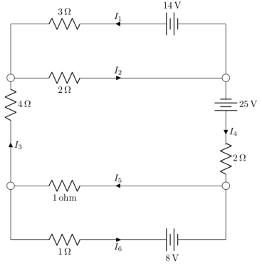
Determine the currents $I_1$, $I_2$, $I_3$, $I_4$, $I_5$, and $I_6$ in the circuit in Figure 3.
Check Your Work
$I_1 = 2\,\textrm{A}$, $I_2 = 4\,\textrm{A}$, $I_3 = 2\,\textrm{A}$, $I_4 = 2\,\textrm{A}$, $I_5 = 5\,\textrm{A}$, $I_6 = 3\,\textrm{A}$.
Follow Along
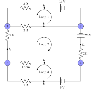
If we designate currents into a node a positive currents, and currents out of the node as negative, applying Kirchoff's first law to the four junctions yields
$$ \begin{align*} \text{Node }1. &\ &I_1+I_3 &= I_2 \\ \text{Node }2. &\ &I_2 &= I_1 + I_4 \\ \text{Node }3. &\ &I_5 &= I_3 + I_6 \\ \text{Node }4. &\ &I_4 + I_6 &= I_5 \end{align*} $$
Applying Kirchoff's second law to the three paths results in
$$ \begin{align*} \text{Loop }1. &\ &3I_1 + 2I_2 &= 14 \\ \text{Loop }2. &\ &2I_2 + 4I_3 + 2I_4 + I_5 &= 25 \\ \text{Loop }3. &\ &I_5 + I_6 &= 8 \end{align*} $$
This is an overdetermined linear system
$$ \begin{align*} \begin{bmatrix}\ \ 1\ & -1\ &\ \ 1\ &\ \ 0\ &\ \ 0\ &\ \ 0\ & | &\ \ 0\ \\ \ \ 1\ & -1\ &\ \ 0\ &\ \ 1\ &\ \ 0\ &\ \ 0\ & | &\ \ 0\ \\ \ \ 0\ &\ \ 0\ &\ \ 1\ &\ \ 0\ & -1\ &\ \ 1\ & | &\ \ 0\ \\ \ \ 0\ &\ \ 0\ &\ \ 0\ &\ \ 1\ & -1\ &\ \ 1\ & | & \ \ 0\ \\ \ \ 3\ &\ \ 2\ &\ \ 0\ &\ \ 0\ &\ \ 0\ &\ \ 0\ & | &\ \,14\ \\ \ \ 0\ &\ \ 2\ &\ \ 4\ &\ \ 2\ &\ \ 1\ &\ \ 0\ & | &\ \,25\ \\ \ \ 0\ &\ \ 0\ &\ \ 0\ &\ \ 0\ &\ \ 1\ &\ \ 1\ & | &\ \ 8\ \end{bmatrix}\begin{array}{l} \\ R_2-R_1 \\ \\ \\ R_5-3R_1 \\ \\ \\ \end{array} &\rightarrow\begin{bmatrix}\ \ 1\ & -1\ &\ \ 1\ &\ \ 0\ &\ \ 0\ &\ \ 0\ & | &\ \ 0\ \\ \ \ 0\ &\ \ 0\ & -1\ &\ \ 1\ &\ \ 0\ &\ \ 0\ & | &\ \ 0\ \\ \ \ 0\ &\ \ 0\ &\ \ 1\ &\ \ 0\ & -1\ &\ \ 1\ & | &\ \ 0\ \\ \ \ 0\ &\ \ 0\ &\ \ 0\ &\ \ 1\ & -1\ &\ \ 1\ & | & \ \ 0\ \\ \ \ 0\ &\ \ 5\ & -3\ &\ \ 0\ &\ \ 0\ &\ \ 0\ & | &\ \,14\ \\ \ \ 0\ &\ \ 2\ &\ \ 4\ &\ \ 2\ &\ \ 1\ &\ \ 0\ & | &\ \,25\ \\ \ \ 0\ &\ \ 0\ &\ \ 0\ &\ \ 0\ &\ \ 1\ &\ \ 1\ & | &\ \ 8\ \end{bmatrix}\begin{array}{l} \\ \\ \\ \\ R_5-2R_6 \\ \\ \\ \end{array} \\ \\ \rightarrow\begin{bmatrix}\ \ 1\ & -1\ &\ \ 1\ &\ \ 0\ &\ \ 0\ &\ \ 0\ & | &\ \ 0\ \\ \ \ 0\ &\ \ 0\ & -1\ &\ \ 1\ &\ \ 0\ &\ \ 0\ & | &\ \ 0\ \\ \ \ 0\ &\ \ 0\ &\ \ 1\ &\ \ 0\ & -1\ &\ \ 1\ & | &\ \ 0\ \\ \ \ 0\ &\ \ 0\ &\ \ 0\ &\ \ 1\ & -1\ &\ \ 1\ & | & \ \ 0\ \\ \ \ 0\ &\ \ 1\ & -11\ & -4\ & -2\ &\ \ 0\ & | & -36\ \\ \ \ 0\ &\ \ 2\ &\ \ 4\ &\ \ 2\ &\ \ 1\ &\ \ 0\ & | &\ \,25\ \\ \ \ 0\ &\ \ 0\ &\ \ 0\ &\ \ 0\ &\ \ 1\ &\ \ 1\ & | &\ \ 8\ \end{bmatrix}\begin{array}{l} \\ \\ \\ \\ \\ R_6-2R_5 \\ \\ \end{array} &\rightarrow\begin{bmatrix}\ \ 1\ & -1\ &\ \ 1\ &\ \ 0\ &\ \ 0\ &\ \ 0\ & | &\ \ 0\ \\ \ \ 0\ &\ \ 0\ & -1\ &\ \ 1\ &\ \ 0\ &\ \ 0\ & | &\ \ 0\ \\ \ \ 0\ &\ \ 0\ &\ \ 1\ &\ \ 0\ & -1\ &\ \ 1\ & | &\ \ 0\ \\ \ \ 0\ &\ \ 0\ &\ \ 0\ &\ \ 1\ & -1\ &\ \ 1\ & | & \ \ 0\ \\ \ \ 0\ &\ \ 1\ & -11\ & -4\ & -2\ &\ \ 0\ & | & -36\ \\ \ \ 0\ &\ \ 0\ &\ \,26\ &\ \,10\ &\ \ 5\ &\ \ 0\ & | &\ \,97\ \\ \ \ 0\ &\ \ 0\ &\ \ 0\ &\ \ 0\ &\ \ 1\ &\ \ 1\ & | &\ \ 8\ \end{bmatrix}\begin{array}{l} \\ R_5 \\ \\ \\ R_2 \\ \\ \\ \end{array} \\ \\ \rightarrow\begin{bmatrix}\ \ 1\ & -1\ &\ \ 1\ &\ \ 0\ &\ \ 0\ &\ \ 0\ & | &\ \ 0\ \\ \ \ 0\ &\ \ 1\ & -11\ & -4\ & -2\ &\ \ 0\ & | & -36\ \\ \ \ 0\ &\ \ 0\ &\ \ 1\ &\ \ 0\ & -1\ &\ \ 1\ & | &\ \ 0\ \\ \ \ 0\ &\ \ 0\ &\ \ 0\ &\ \ 1\ & -1\ &\ \ 1\ & | & \ \ 0\ \\ \ \ 0\ &\ \ 0\ & -1\ &\ \ 1\ &\ \ 0\ &\ \ 0\ & | &\ \ 0\ \\ \ \ 0\ &\ \ 0\ &\ \,26\ &\ \,10\ &\ \ 5\ &\ \ 0\ & | &\ \,97\ \\ \ \ 0\ &\ \ 0\ &\ \ 0\ &\ \ 0\ &\ \ 1\ &\ \ 1\ & | &\ \ 8\ \end{bmatrix}\begin{array}{l} \\ \\ \\ \\ R_5+R_3 \\ R_6-26R_3 \\ \\ \end{array} &\rightarrow\begin{bmatrix}\ \ 1\ & -1\ &\ \ 1\ &\ \ 0\ &\ \ 0\ &\ \ 0\ & | &\ \ 0\ \\ \ \ 0\ &\ \ 1\ & -11\ & -4\ & -2\ &\ \ 0\ & | & -36\ \\ \ \ 0\ &\ \ 0\ &\ \ 1\ &\ \ 0\ & -1\ &\ \ 1\ & | &\ \ 0\ \\ \ \ 0\ &\ \ 0\ &\ \ 0\ &\ \ 1\ & -1\ &\ \ 1\ & | & \ \ 0\ \\ \ \ 0\ &\ \ 0\ &\ \ 0\ &\ \ 1\ & -1\ &\ \ 1\ & | &\ \ 0\ \\ \ \ 0\ &\ \ 0\ &\ \ 0\ &\ \,10\ &\ \,31\ & -26\ & | &\ \,97\ \\ \ \ 0\ &\ \ 0\ &\ \ 0\ &\ \ 0\ &\ \ 1\ &\ \ 1\ & | &\ \ 8\ \end{bmatrix}\begin{array}{l} \\ \\ \\ \\ R_5-R_4 \\ R_6-10R_4 \\ \\ \end{array} \\ \end{align*} $$
$$ \begin{align*} \rightarrow\begin{bmatrix}\ \ 1\ & -1\ &\ \ 1\ &\ \ 0\ &\ \ 0\ &\ \ 0\ & | &\ \ 0\ \\ \ \ 0\ &\ \ 1\ & -11\ & -4\ & -2\ &\ \ 0\ & | & -36\ \\ \ \ 0\ &\ \ 0\ &\ \ 1\ &\ \ 0\ & -1\ &\ \ 1\ & | &\ \ 0\ \\ \ \ 0\ &\ \ 0\ &\ \ 0\ &\ \ 1\ & -1\ &\ \ 1\ & | & \ \ 0\ \\ \ \ 0\ &\ \ 0\ &\ \ 0\ &\ \ 0\ &\ \ 0\ &\ \ 0\ & | &\ \ 0\ \\ \ \ 0\ &\ \ 0\ &\ \ 0\ &\ \ 0\ &\ \,41\ & -36\ & | &\ \,97\ \\ \ \ 0\ &\ \ 0\ &\ \ 0\ &\ \ 0\ &\ \ 1\ &\ \ 1\ & | &\ \ 8\ \end{bmatrix}\begin{array}{l} \\ \\ \\ \\ R_7 \\ \\ R_5 \\ \end{array} &\rightarrow\begin{bmatrix}\ \ 1\ & -1\ &\ \ 1\ &\ \ 0\ &\ \ 0\ &\ \ 0\ & | &\ \ 0\ \\ \ \ 0\ &\ \ 1\ & -11\ & -4\ & -2\ &\ \ 0\ & | & -36\ \\ \ \ 0\ &\ \ 0\ &\ \ 1\ &\ \ 0\ & -1\ &\ \ 1\ & | &\ \ 0\ \\ \ \ 0\ &\ \ 0\ &\ \ 0\ &\ \ 1\ & -1\ &\ \ 1\ & | & \ \ 0\ \\ \ \ 0\ &\ \ 0\ &\ \ 0\ &\ \ 0\ &\ \ 1\ &\ \ 1\ & | &\ \ 8\ \\ \ \ 0\ &\ \ 0\ &\ \ 0\ &\ \ 0\ &\ \,41\ & -36\ & | &\ \,97\ \\ \ \ 0\ &\ \ 0\ &\ \ 0\ &\ \ 0\ &\ \ 0\ &\ \ 0\ & | &\ \ 0\ \end{bmatrix}\begin{array}{l} \\ \\ \\ \\ \\ R_6-41R_5 \\ \\ \end{array} \\ \\ \rightarrow\begin{bmatrix}\ \ 1\ & -1\ &\ \ 1\ &\ \ 0\ &\ \ 0\ &\ \ 0\ & | &\ \ 0\ \\ \ \ 0\ &\ \ 1\ & -11\ & -4\ & -2\ &\ \ 0\ & | & -36\ \\ \ \ 0\ &\ \ 0\ &\ \ 1\ &\ \ 0\ & -1\ &\ \ 1\ & | &\ \ 0\ \\ \ \ 0\ &\ \ 0\ &\ \ 0\ &\ \ 1\ & -1\ &\ \ 1\ & | & \ \ 0\ \\ \ \ 0\ &\ \ 0\ &\ \ 0\ &\ \ 0\ &\ \ 1\ &\ \ 1\ & | &\ \ 8\ \\ \ \ 0\ &\ \ 0\ &\ \ 0\ &\ \ 0\ &\ \ 0\ & -77\ & | & -231\ \\ \ \ 0\ &\ \ 0\ &\ \ 0\ &\ \ 0\ &\ \ 0\ &\ \ 0\ & | &\ \ 0\ \end{bmatrix}\begin{array}{l} \\ \\ \\ \\ \\ -\frac{1}{77}R_6 \\ \\ \end{array} &\rightarrow\begin{bmatrix}\ \ 1\ & -1\ &\ \ 1\ &\ \ 0\ &\ \ 0\ &\ \ 0\ & | &\ \ 0\ \\ \ \ 0\ &\ \ 1\ & -11\ & -4\ & -2\ &\ \ 0\ & | & -36\ \\ \ \ 0\ &\ \ 0\ &\ \ 1\ &\ \ 0\ & -1\ &\ \ 1\ & | &\ \ 0\ \\ \ \ 0\ &\ \ 0\ &\ \ 0\ &\ \ 1\ & -1\ &\ \ 1\ & | & \ \ 0\ \\ \ \ 0\ &\ \ 0\ &\ \ 0\ &\ \ 0\ &\ \ 1\ &\ \ 1\ & | &\ \ 8\ \\ \ \ 0\ &\ \ 0\ &\ \ 0\ &\ \ 0\ &\ \ 0\ &\ \ 1\ & | &\ \ 3\ \\ \ \ 0\ &\ \ 0\ &\ \ 0\ &\ \ 0\ &\ \ 0\ &\ \ 0\ & | &\ \ 0\ \end{bmatrix}\begin{array}{l} \\ \\ R_3-R_6 \\ R_4-R_6 \\ R_5-R_6 \\ \\ \\ \end{array} \\ \\ \rightarrow\begin{bmatrix}\ \ 1\ & -1\ &\ \ 1\ &\ \ 0\ &\ \ 0\ &\ \ 0\ & | &\ \ 0\ \\ \ \ 0\ &\ \ 1\ & -11\ & -4\ & -2\ &\ \ 0\ & | & -36\ \\ \ \ 0\ &\ \ 0\ &\ \ 1\ &\ \ 0\ & -1\ &\ \ 0\ & | & -3\ \\ \ \ 0\ &\ \ 0\ &\ \ 0\ &\ \ 1\ & -1\ &\ \ 0\ & | & -3\ \\ \ \ 0\ &\ \ 0\ &\ \ 0\ &\ \ 0\ &\ \ 1\ &\ \ 0\ & | &\ \ 5\ \\ \ \ 0\ &\ \ 0\ &\ \ 0\ &\ \ 0\ &\ \ 0\ &\ \ 1\ & | &\ \ 3\ \\ \ \ 0\ &\ \ 0\ &\ \ 0\ &\ \ 0\ &\ \ 0\ &\ \ 0\ & | &\ \ 0\ \end{bmatrix}\begin{array}{l} \\ R_2+2R_5 \\ R_3+R_5 \\ R_4+R_5 \\ \\ \\ \\ \end{array} &\rightarrow\begin{bmatrix}\ \ 1\ & -1\ &\ \ 1\ &\ \ 0\ &\ \ 0\ &\ \ 0\ & | &\ \ 0\ \\ \ \ 0\ &\ \ 1\ & -11\ & -4\ &\ \ 0\ &\ \ 0\ & | & -26\ \\ \ \ 0\ &\ \ 0\ &\ \ 1\ &\ \ 0\ &\ \ 0\ &\ \ 0\ & | &\ \ 2\ \\ \ \ 0\ &\ \ 0\ &\ \ 0\ &\ \ 1\ &\ \ 0\ &\ \ 0\ & | &\ \ 2\ \\ \ \ 0\ &\ \ 0\ &\ \ 0\ &\ \ 0\ &\ \ 1\ &\ \ 0\ & | &\ \ 5\ \\ \ \ 0\ &\ \ 0\ &\ \ 0\ &\ \ 0\ &\ \ 0\ &\ \ 1\ & | &\ \ 3\ \\ \ \ 0\ &\ \ 0\ &\ \ 0\ &\ \ 0\ &\ \ 0\ &\ \ 0\ & | &\ \ 0\ \end{bmatrix}\begin{array}{l} \\ R_2+4R_4 \\ \\ \\ \\ \\ \\ \end{array} \\ \end{align*} $$
$$ \begin{align*} \rightarrow\begin{bmatrix}\ \ 1\ & -1\ &\ \ 1\ &\ \ 0\ &\ \ 0\ &\ \ 0\ & | &\ \ 0\ \\ \ \ 0\ &\ \ 1\ & -11\ &\ \ 0\ &\ \ 0\ &\ \ 0\ & | & -18\ \\ \ \ 0\ &\ \ 0\ &\ \ 1\ &\ \ 0\ &\ \ 0\ &\ \ 0\ & | &\ \ 2\ \\ \ \ 0\ &\ \ 0\ &\ \ 0\ &\ \ 1\ &\ \ 0\ &\ \ 0\ & | &\ \ 2\ \\ \ \ 0\ &\ \ 0\ &\ \ 0\ &\ \ 0\ &\ \ 1\ &\ \ 0\ & | &\ \ 5\ \\ \ \ 0\ &\ \ 0\ &\ \ 0\ &\ \ 0\ &\ \ 0\ &\ \ 1\ & | &\ \ 3\ \\ \ \ 0\ &\ \ 0\ &\ \ 0\ &\ \ 0\ &\ \ 0\ &\ \ 0\ & | &\ \ 0\ \end{bmatrix}\begin{array}{l} R_1-R_3 \\ R_2+11R_3 \\ \\ \\ \\ \\ \\ \end{array} &\rightarrow\begin{bmatrix}\ \ 1\ & -1\ &\ \ 0\ &\ \ 0\ &\ \ 0\ &\ \ 0\ & | & -2\ \\ \ \ 0\ &\ \ 1\ &\ \ 0\ &\ \ 0\ &\ \ 0\ &\ \ 0\ & | &\ \ 4\ \\ \ \ 0\ &\ \ 0\ &\ \ 1\ &\ \ 0\ &\ \ 0\ &\ \ 0\ & | &\ \ 2\ \\ \ \ 0\ &\ \ 0\ &\ \ 0\ &\ \ 1\ &\ \ 0\ &\ \ 0\ & | &\ \ 2\ \\ \ \ 0\ &\ \ 0\ &\ \ 0\ &\ \ 0\ &\ \ 1\ &\ \ 0\ & | &\ \ 5\ \\ \ \ 0\ &\ \ 0\ &\ \ 0\ &\ \ 0\ &\ \ 0\ &\ \ 1\ & | &\ \ 3\ \\ \ \ 0\ &\ \ 0\ &\ \ 0\ &\ \ 0\ &\ \ 0\ &\ \ 0\ & | &\ \ 0\ \end{bmatrix}\begin{array}{l} R_1+R_2 \\ \\ \\ \\ \\ \\ \\ \end{array} \\ \\ \rightarrow\begin{bmatrix}\ \ 1\ &\ \ 0\ &\ \ 0\ &\ \ 0\ &\ \ 0\ &\ \ 0\ & | &\ \ 2\ \\ \ \ 0\ &\ \ 1\ &\ \ 0\ &\ \ 0\ &\ \ 0\ &\ \ 0\ & | &\ \ 4\ \\ \ \ 0\ &\ \ 0\ &\ \ 1\ &\ \ 0\ &\ \ 0\ &\ \ 0\ & | &\ \ 2\ \\ \ \ 0\ &\ \ 0\ &\ \ 0\ &\ \ 1\ &\ \ 0\ &\ \ 0\ & | &\ \ 2\ \\ \ \ 0\ &\ \ 0\ &\ \ 0\ &\ \ 0\ &\ \ 1\ &\ \ 0\ & | &\ \ 5\ \\ \ \ 0\ &\ \ 0\ &\ \ 0\ &\ \ 0\ &\ \ 0\ &\ \ 1\ & | &\ \ 3\ \\ \ \ 0\ &\ \ 0\ &\ \ 0\ &\ \ 0\ &\ \ 0\ &\ \ 0\ & | &\ \ 0\ \end{bmatrix} \end{align*} $$
The seventh row is identically zero, showing that one of our seven equations was redundant — the four node equations are linearly dependent. Hence our unique solution for the currents across each resistor are
$$I_1 = 2\,\textrm{A},\ I_2 = 4\,\textrm{A},\ I_3 = 2\,\textrm{A},\ I_4 = 2\,\textrm{A},\ I_5 = 5\,\textrm{A},\ I_6 = 3\,\textrm{A}$$
1.3.4 Short Answer Exercises
Short Answer Exercises
Exercise 5 - Homogeneous Linear Equations
Given a homogeneous linear system of equations, if the system is overdetermined, what are the possibilities for the number of solutions to the linear system?
Check Your Work
Either exactly one solution (the zero vector) or infinitely many. Never none.
Follow Along
A homogeneous linear system of equations is always consistent because the zero vector is always a solution. An overdetermined linear system may be either dependent or independent. Consider the following simple examples of $3\times 2$ matrices in reduced row echelon form.
$$ A = \begin{bmatrix} 1 & 0 \\ 0 & 0 \\ 0 & 0 \end{bmatrix} \qquad B = \begin{bmatrix} 1 & 0 \\ 0 & 1 \\ 0 & 0 \end{bmatrix} $$
Matrix $A$ has a free column, so the homogeneous linear system is dependent. The homogeneous linear system $A\mathbf{x}=\mathbf{0}$ has infinitely many solutions, $\left\{\, \begin{bmatrix}\ -s\ \\ \ \ s\ \end{bmatrix} \,:\, s\in\mathbb{R} \,\right\}$.
Matrix $B$ has no free column, so the homogeneous linear system is independent. The homogeneous linear system $B\mathbf{x}=\mathbf{0}$ has only one solution, $\left\{ \begin{bmatrix}\ 0\ \\ \ 0\ \end{bmatrix} \right\}$.
Exercise 6 - Homogeneous Geometric Explanation
Give a geometric explanation why a homogeneous linear system consisting of two equations with three unknowns must have infinitely many solutions.
Check Your Work
The two planes either coincide or meet in a line, so there are infinitely many common points.
Follow Along
The graph of a homogeneous linear system consisting of two equations with three unknowns is two planes. These two planes that share at least one point are either the same plane, or intersect in a line. In either case there are infinitely many points that lie on both planes, so the linear system has infinitely many solutions.
Exercise 7 - A Linear System with Two Solutions
Let $A\mathbf{x}=\mathbf{b}$ be a system of $n$ linear equations with $n$ unknowns, and suppose that the linear system has two distinct solutions $\mathbf{x}_1\neq\mathbf{x}_2$. Explain how many solutions the linear system $A\mathbf{x}=\mathbf{b}$ must have.
Check Your Work
Infinitely many solutions.
Follow Along
The only possible number of solutions of a linear system of equations are
- no solutions (inconsistent)
- infinitely many solutions (dependent and consistent)
- only one solution (independent and consistent)
Given that the linear system has two solutions $\mathbf{x}_1$ and $\mathbf{x}_2$, the linear system is consistent. Since there are more than one solution, the only possibility is infinitely many solutions.
1.3.5 True/False Questions
State and explain whether the following statement is true or false.
If true explain why the statement is true. If false provide a counter-example that shows the statement is false.
Check Your Work
1. False. 2. False. 3. False. 4. True. 5. True.
6. True. 7. True. 8. True. 9. True. 10. True.
- If $m\times n$ matrix $A$ has a free column, then linear system $A\mathbf{x}=\mathbf{b}$ will have infinitely many solutions.
Follow Along
False. Since matrix $A$ has a free column, the linear system is dependent. However there are still two possibilities. If the linear system is consistent, then it has infinitely many solutions. However if the linear system is inconsistent, then the linear system has no solutions. Consider the augmented matrix
$$ \begin{bmatrix}\ 1\ &\ 0\ & | &\ 0\ \\ \ 0\ &\ 0\ & | &\ 1\ \end{bmatrix} $$
The augmented matrix represents a linear system that has no solutions.
- If a linear system has more equations than unknowns, then the system must be inconsistent.
Follow Along
False. The system is overdetermined, which makes inconsistency typical but not guaranteed. If some equations are linear combinations of others, the system can be consistent and even have a unique solution. Example: three copies of the equation $x+y=1$ form a $3 \times 2$ system with infinitely many solutions.
- If a linear system has fewer equations than unknowns, then the system must have infinitely many solutions.
Follow Along
False. Underdetermined systems can still be inconsistent. Example: $x + y + z = 1$ and $x + y + z = 2$ is a $2\times3$ underdetermined example that has no solution despite having two equations in three unknowns.
- Every homogeneous linear system has at least one solution.
Follow Along
True. The zero vector $\mathbf{x} = \mathbf{0}$ satisfies $A\mathbf{x} = \mathbf{0}$ for any matrix $A$. A homogeneous system is always consistent.
- If two row vectors $\mathbf{a}_1$ and $\mathbf{a}_2$ are scalar multiples of one another, then the linear system whose coefficient matrix has these two rows is dependent.
Follow Along
True. If $\mathbf{a}_2 = c\mathbf{a}_1$ for some scalar $c$, then row reduction will produce a zero row, signaling a free column or a redundant equation. The system is dependent in the row picture.
- If $A\mathbf{x} = \mathbf{b}$ has a unique solution, then $A\mathbf{x} = \mathbf{0}$ also has a unique solution.
Follow Along
True. If $A\mathbf{x} = \mathbf{b}$ has a unique solution, the coefficient matrix has no free columns. The same coefficient matrix in the homogeneous system $A\mathbf{x} = \mathbf{0}$ therefore also has no free columns, so the only solution is the zero vector.
- If $A$ is an $n\times n$ matrix and every column of $A$ is a pivot column, then $A\mathbf{x} = \mathbf{b}$ has a unique solution for every choice of $\mathbf{b}$.
Follow Along
True. If $A$ has $n$ pivots and $n$ columns, there are no free columns; the reduced row echelon form has a $1$ in every column. Whatever the right-hand side, back-substitution gives exactly one solution.
- A matrix in reduced row echelon form is also in upper triangular form.
Follow Along
True. Any matrix in reduced row echelon form is in row echelon form as well. A matrix in row echelon form is a matrix in upper triangular form with pivot values that are not necessarily one.
- If $\mathbf{x}_1$ and $\mathbf{x}_2$ are two distinct solutions of $A\mathbf{x} = \mathbf{b}$, then $\mathbf{x}_1 - \mathbf{x}_2$ is a solution of the homogeneous system $A\mathbf{x} = \mathbf{0}$.
Follow Along
True. Computing directly: $A(\mathbf{x}_1 - \mathbf{x}_2) = A\mathbf{x}_1 - A\mathbf{x}_2 = \mathbf{b} - \mathbf{b} = \mathbf{0}$. This is the foundational fact behind the particular solution plus homogeneous solution form of a solution.
- If $A$ is an $m\times n$ matrix with $m < n$, then the homogeneous system $A\mathbf{x} = \mathbf{0}$ must have a nonzero solution.
Follow Along
True. The system is underdetermined and homogeneous, so it is consistent (the zero vector works) and has more unknowns than equations. After row reduction, at least one column of $A$ is a free column, producing a free variable that can take any nonzero value while the rest adjust accordingly. The solution set is at least a line that passes through this nonzero solution vector $\mathbf{v}$ and the trivial solution $\mathbf{0}$.
1.3.6 Multiple Choice Questions
Check All That Apply
Each question below may have more than one correct choice. Check every box that applies. No justification is required.
1. A rational function is decomposed as a sum of partial fractions and the coefficients are found by equating polynomials. Which of the following are true?
$\square\ $ The resulting equations in the unknown coefficients are linear
$\square\ $ A repeated linear factor $(x-a)^2$ contributes two terms
$\square\ $ The method requires factoring the denominator first
$\square\ $ The resulting linear system is always homogeneous
$\square\ $ The number of unknowns equals the degree of the denominator
2. Which of the following are true of the linear system that balances a chemical reaction?
$\square\ $ It is homogeneous
$\square\ $ It is always inconsistent
$\square\ $ It has one equation for each element in the reaction
$\square\ $ Only its integer solutions are chemically meaningful
$\square\ $ The zero vector is a solution but is not a balanced equation
3. Let $P$ be a transition of probabilities matrix. Which of the following are true?
$\square\ $ Every entry lies in $[0,1]$
$\square\ $ Each column sums to one
$\square\ $ Each row sums to one
$\square\ $ $P^2$ is also a transition of probabilities matrix
$\square\ $ $P$ must be square to be applied twice
4. A network flow problem is modeled with flow in equal to flow out at every node. Which of the following are true?
$\square\ $ Each node contributes one linear equation
$\square\ $ The node equations can be linearly dependent
$\square\ $ The system can be underdetermined, leaving a free variable
$\square\ $ Negative values of a flow variable are always meaningful
$\square\ $ The system is always square
Check Your Work
1. The first, second, and third.
2. The first, third, fourth, and fifth.
3. The first, second, fourth, and fifth.
4. The first, second, and third.
1.3.7 Challenge Exercises
Problems Spanning the Whole Section
These exercises combine the modeling steps of this section with the elimination methods of 1.2. Only the answers are given; producing the argument is the exercise.
Exercise 8 - Balancing a Harder Reaction
Propane burns completely in oxygen to produce carbon dioxide and water.
$$ x_1C_3H_8 + x_2O_2 \longrightarrow x_3CO_2 + x_4H_2O $$
Set up the homogeneous linear system, reduce the coefficient matrix to Hermite normal form, and determine the smallest positive integer solution.
Check Your Work
$x_1 = 1$, $x_2 = 5$, $x_3 = 3$, $x_4 = 4$, giving
$$ C_3H_8 + 5O_2 \longrightarrow 3CO_2 + 4H_2O $$
Exercise 9 - A Partial Fraction Decomposition with a Parameter
Consider the decomposition
$$ \dfrac{x + a}{(x-2)(x+3)} = \dfrac{A}{x-2} + \dfrac{B}{x+3} $$
(a) Write the linear system satisfied by $A$ and $B$ in terms of the constant $a$.
(b) Solve for $A$ and $B$.
(c) For which value of $a$ does the decomposition reduce to a single term?
Check Your Work
(a) $A + B = 1$ and $3A - 2B = a$.
(b) $A = \dfrac{a+2}{5}$ and $B = \dfrac{3-a}{5}$.
(c) $a = -2$ kills the first term and $a = 3$ kills the second.
Exercise 10 - A Network That Cannot Be Balanced
A network has three nodes. Node $a$ receives $30$ units from outside and sends $x_1$ to node $b$ and $x_2$ to node $c$. Node $b$ sends $x_3$ to node $c$ and discharges $10$ units outside. Node $c$ discharges $k$ units outside.
(a) Write the node equations.
(b) Determine the value of $k$ for which the system is consistent.
(c) For that value of $k$, describe the solution set and determine which solutions have all flows nonnegative.
Check Your Work
(a) $x_1 + x_2 = 30$, $x_1 = x_3 + 10$, $x_2 + x_3 = k$.
(b) $k = 20$.
(c) A one-parameter family with $x_3 = t$, $x_1 = t + 10$, and $x_2 = 20 - t$; all flows are nonnegative for $0 \le t \le 20$.
Creative Commons License
Mathematics, Statistics & Physics
Your use of this self-initiated mediated course material is subject to our Creative Commons License 4.0