
Video Lecture 1: Vectors in ℝⁿ
 Vectors in ℝⁿ
A vector on the plane has two quantities associated with it; its magnitude and direction.
The magnitude of a vector in $\mathbb{R}^2$ is the length of the vector, and the direction of such a vector is the angle the vector makes with a vector parallel to $\ihat$.
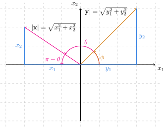
Notice that this definition does not include where the vector is located on the plane.
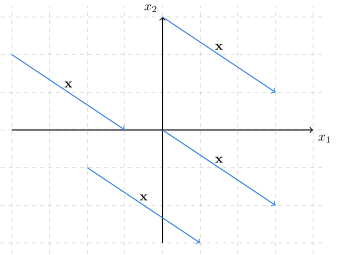
All of the vectors in figure 2 are the same vector! In some applications one says that the vector is applied at a specific point $P = (x_0,y_0,z_0)$ if the terminal point of the vector is located at $P$. However the same vector can be applied to any point on the plane.
The coordinates of a vector on the plane are the coordinates of the tip of the vector when the base of the vector is the origin, $(0,0)$; when the initial point of a vector is the origin. Such a vector is said to be in standard position. In figure 1, both vectors $\mathbf{x}$ and $\mathbf{y}$ are in standard position.
The standard coordinates of a vector are the coordinates of the tip of the vector in standard position. Often we denote the coordinates of a vector using the same lower case letter in normal font to indicate it is a scalar, and with a subscript to indicate which coordinate it is.
$$ \mathbf{v} = \begin{bmatrix} v_1 \\ v_2 \end{bmatrix} = \langle v_1, v_2 \rangle $$
The coordinates are also called the scalar components of the vector since the linear combination of the standard basis vectors, $\ihat$ and $\jhat$ are given by
$$ \mathbf{v} = v_1\ihat + v_2\jhat = v_1\mathbf{e}_1 + v_2\mathbf{e}_2 $$
We will soon be discussing vectors in $\mathbb{R}^n$. In $\mathbb{R}^2$ and $\mathbb{R}^3$ we typically denote the standard basis vectors by $\ihat$, $\jhat$, and $\khat$. For large $n$ we need a more flexible notation. The standard basis vectors in $\mathbb{R}^n$ are $\mathbf{e}_1$, $\mathbf{e}_2$, $\mathbf{e}_3$, $\dots$, $\mathbf{e}_n$. Thus in $\mathbb{R}^3$,
$$\ihat = \mathbf{e}_1,\ \jhat = \mathbf{e}_2,\ \khat = \mathbf{e}_3$$
Suppose $\mathbf{x}$ is a vector in $\mathbb{R}^2$. The vector may be considered as both an arrow from the origin to a point $(x_1,x_2)$ and a list of numbers
$$\mathbf{x} = \begin{bmatrix} x_1 \\ x_2 \end{bmatrix}. $$
If $x_1 = 3$ and $x_2 = -2$, then graphically we have
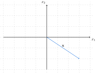
To find the magnitude of a vector $\|\mathbf{x}\|$, we compute the Euclidean distance $d$ from the base to the tip of the vector.
$$ \|\mathbf{x}\| := d = \sqrt{x_1^2 + x_2^2}. $$
This formula should remind you of the Pythagorean theorem.
The angle between two vectors $\mathbf{x}$ and $\mathbf{y}$ is given using dot product and the formula
$$ \cos\theta = \dfrac{\mathbf{x}\cdot\mathbf{y}}{\|\mathbf{x}\|\|\mathbf{y}\|} $$
Exercise 1 - Find Magnitude and Angle
If $\mathbf{x} = \begin{bmatrix} 1 \\ 3 \end{bmatrix}$ and $\mathbf{y} = \begin{bmatrix} 0 \\ 2 \end{bmatrix}$, what is $\|\mathbf{x}\|$, $\|\mathbf{y}\|$, and the angle between these two vectors in $\mathbb{R}^2$?
View Solution
$$ \begin{align*} \|\mathbf{x}\| &= \sqrt{ 1^2 + 3^2 } = \sqrt{1 + 9 } =\sqrt{10} \\ \\ \|\mathbf{y}\| &= \sqrt{ 0^2 + 2^2 } = \sqrt{ 0 + 4 } = \sqrt{4} = 2 \\ \\ \cos\left(\theta\right) &= \dfrac{\mathbf{x}\cdot\mathbf{y}}{\|\mathbf{x}\|\|\mathbf{y}\|} = \dfrac{ 1(0) + 3(2) }{ \sqrt{10}\cdot 2 } = \frac{3}{\sqrt{10}} \\ \\ \theta &= \cos^{-1}\left(\frac{3}{\sqrt{10}}\right) \end{align*} $$
The most important concept in linear algebra is the idea of a linear combination. Linear combinations and the properties of vector spaces arise from scalar multiplication and vector addition.
Definition
2D Scalar Multiplication
Scalar multiplication quite literally scales a vector's magnitude by a constant. Most times, these scalars are real numbers, but in some vector spaces they are complex numbers. You are probably already familiar with the computer scientist's perspective in $\mathbb{R}^2$. Let $t$ be some real number, then
$$ t\mathbf{x} = t\begin{bmatrix} x_1 \\ x_2 \end{bmatrix} = \begin{bmatrix} t x_1 \\ t x_2 \end{bmatrix}. $$
If $t \gt 0$, then $t\mathbf{x}$ is a vector whose magnitude is now $t$ times the magnitude of $\mathbf{x}$.
If $t \lt 0$, then $t$ scales magnitude by $|t|$, and $t\mathbf{x}$ points in the opposite direction of $\mathbf{x}$.
If $|t|\gt 1$, then the scalar stretches or dilates the magnitude of the vector.
If $0 \lt |t| \lt 1$, then the scalar shrinks or contracts the magnitude of the vector.
Multiplying a vector by the scalar $0$ yields the zero vector $\mathbf{0}$.
Multiplying a vector by $1$ has no effect on the vector.
Using the physicist picture, this looks like
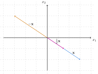
For the above image, we have vector $\mathbf{x} = \begin{bmatrix}\ \ 3 \\ -2 \end{bmatrix}$,
$$ \frac{1}{2}\mathbf{x} = \frac{1}{2}\begin{bmatrix}\ \ 3 \\ -2 \end{bmatrix} = \begin{bmatrix} \frac{3}{2} \\ -1 \end{bmatrix} $$
and
$$ -\mathbf{x} = (-1)\left[\begin{array}{cc} 3 \\ -2 \end{array}\right] = \left[\begin{array}{cc} -3 \\ 2 \end{array}\right]. $$
Definition
2D Vector Addition
Vector addition is computed component-wise from the computer scientist's perspective. If you have two vectors $\mathbf{x}$ and $\mathbf{y}$, their vector sum is
$$ \mathbf{x} + \mathbf{y} = \begin{bmatrix} x_1 \\ x_2 \end{bmatrix} + \begin{bmatrix} y_1 \\ y_2 \end{bmatrix} = \begin{bmatrix} x_1 + y_1 \\ x_2 + y_2 \end{bmatrix}. $$
From the physicist perspective, vector addition is commonly described using the term triangle law. This is because if the vectors $\mathbf{x}$ and $\mathbf{y}$ are arranged so that the tail of $\mathbf{x}$ is at the origin and the tail of $\mathbf{y}$ sits at the tip of $\mathbf{x}$, then the sum of those vectors is the directed line segment from the origin to $\mathbf{y}$'s tip.
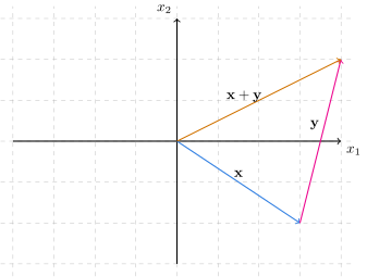
The commutative property of vector addition
$$ \mathbf{x} + \mathbf{y} = \mathbf{y} + \mathbf{x} $$
may be demonstrated visually as well by forming a parallelogram
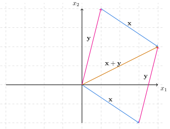
This is simply drawing both possible triangles for vector addition. The combination of those two triangles forming a parallelogram. Heuristically, this leads to people describing vector addition as tip to tail.
We focused on $\mathbb{R}^2$ here, but the above description and properties work for all $\mathbb{R}^n$, with more complicated pictures.
Exercise 2 - Evaluate Vector Expression
If $\mathbf{x} = \begin{bmatrix} 1 \\ 3 \end{bmatrix}$ and $\mathbf{y} = \begin{bmatrix} 0 \\ 2 \end{bmatrix}$, what is the vector $2\mathbf{x} - 3\mathbf{y}$?
View Solution
$$ \begin{align*} 2\mathbf{x} - 3\mathbf{y} &= 2\begin{bmatrix} 1 \\ 3 \end{bmatrix} - 3\begin{bmatrix} 0 \\ 2 \end{bmatrix} = \begin{bmatrix} 2 \\ 6 \end{bmatrix} - \begin{bmatrix} 0 \\ 6 \end{bmatrix} = \begin{bmatrix} 2-0 \\ 6-6 \end{bmatrix} = \begin{bmatrix} 2 \\ 0 \end{bmatrix} \\ \end{align*} $$Video Lecture 2: Three Dimensional Vectors and Transformations.
 Three Dimensional Vectors and Transformations
In $\mathbb{R}^2$, vector addition and scalar multiplication share many algebraic properties with matrices. Vectors in $\mathbb{R}^n$ share these same properties. It is more useful to use Grant Sanderson's computer scientist's perspective of a vector when the number of dimensions is greater than $3$. The computer scientist views vectors as a column of numbers. We shall see in chapter 5 that vectors in $\mathbb{R}^n$ share the geometrical properties of 2D and 3D vectors.
Video Lecture 3: Vector Space ℝⁿ.
Vector Space ℝⁿ
Definition
Vector Space $\mathbb{R}^n$
Vector Space $\mathbb{R}^n$ is the set of all ordered $n$-tuples of real numbers. To distinguish vectors in $\mathbb{R}^n$ from points in $n$-dimensional Real coordinate space, vectors are denoted by an $n\times 1$ matrix,
$$\mathbf{x} = \begin{bmatrix} x_1 \\ \vdots \\ x_n \end{bmatrix} = \begin{pmatrix} x_1 \\ \vdots \\ x_n \end{pmatrix}$$
Angle brackets may also be used, although angle brackets are also used to denote inner product. This makes it a less attractive notation. Finally one may save space by writing a vector as the transpose of a $1\times n$ matrix,
$$\mathbf{x} = \begin{bmatrix} x_1 & \cdots & x_n \end{bmatrix}^\mathsf{T}.$$
Vector addition and scalar multiplication of vectors is defined axiomatically as follows:
Let $\mathbf{u}$ and $\mathbf{v}$ be vectors in $\mathbb{R}^n$ and $c$ is a real scalar, then
Vector Addition and Scalar Multiplication are defined element-wise:
$\mathbf{u} + \mathbf{v} = \left[ u_i \right] + \left[ v_i \right] = \left[ u_i + v_i \right]\in\mathbb{R}^n$
$c\mathbf{u} = c\left[ u_i \right] = \left[ cu_i \right]\in\mathbb{R}^n$
Together these properties are called the closure properties because they state that the sum of two vectors in $\mathbb{R}^n$ is a vector in $\mathbb{R}^n$, and defines how to add them. Likewise, they state that the scalar multiple of a vector in $\mathbb{R}^n$ is a vector in $\mathbb{R}^n$, and it defines how to compute the scalar multiple.
One may demonstrate the algebraic properties of vector space $\mathbb{R}^n$ using the same short notation we developed for matrices. However vectors in $\mathbb{R}^n$ require only one subscript to identify each element.
Historically, matrices pre-date modern notation for vectors. The definition of vectors was developed by
Josiah Willard Gibbs,
Oliver Heaviside, and others. Over a thousand years earlier Chinese mathematicians developed the
Fangcheng method for solving systems of linear equations using what we call Gaussian elimination.
These properties of vectors give us a framework to denote mathematical objects that describe Euclidean geometry. Vectors are used to describe force, dynamic state, heat flux, charge density, probability, inertia, torque, spinors, velocity, and acceleration. This is a small sample of the applications of vectors in modern physics. The algebraic axioms of the definition of vectors in $\mathbb{R}^n$ are precisely the algebraic properties of the basic quantities of physics they are designed to represent.
Theorem 1
Algebraic Properties of $\mathbb{R}^n$
For all vectors $\mathbf{u}$, $\mathbf{v}$, and $\mathbf{w}$ in $\mathbb{R}^n$, and real scalars $c$ and $d$:
$\mathbf{u} + \mathbf{v} = \mathbf{v} + \mathbf{u}$
$( \mathbf{u} + \mathbf{v} ) + \mathbf{w} = \mathbf{u} + ( \mathbf{v} + \mathbf{w} )$
$\mathbf{0} = \left[ 0, \dots, 0 \right]^\mathsf{T}$ is the additive identity, $\mathbf{0} + \mathbf{u} = \mathbf{u} + \mathbf{0} = \mathbf{u}$
$(-1)\mathbf{u}$ is the additive inverse, $(-1)\mathbf{u} + \mathbf{u} = \mathbf{u} + (-1)\mathbf{u} = \mathbf{0}$
$c(\mathbf{u} + \mathbf{v}) = c\mathbf{u} + c\mathbf{v}$
$(c + d)\mathbf{u} = c\mathbf{u} + d\mathbf{u}$
$(cd)\mathbf{u} = c\left(d\mathbf{u}\right)$
$(1)\mathbf{u} = \mathbf{u}$
Proof of Theorem 1-1
For all vectors $\mathbf{u}$ and $\mathbf{v}$ in $\mathbb{R}^n$,
$$ \mathbf{u} + \mathbf{v} = [ u_i ] + [ v_i ] = [ u_i + v_i ] = [ v_i + u_i ] = [ v_i ] + [ u_i ] = \mathbf{v} + \mathbf{u}.\ \blacksquare $$
All of these properties are derived from the algebraic properties of real numbers. We used the above notation in similar proofs concerning the algebraic properties of matrix addition and scalar multiplication in chapter 2. Students should be able to produce the proofs of all $8$ of these properties.
Exercise 3 - Evaluate Vector Expressions
Let $\mathbf{u} = \langle -4, -2, 1 \rangle$ and $\mathbf{v} = \langle 0, 3, -4 \rangle$
Determine the magnitudes of $\mathbf{u}$, $\mathbf{v}$, and $\mathbf{u} + \mathbf{v}$
Perform each vector operation
(a) $2\mathbf{u} + \mathbf{v}$
(b) $5\mathbf{v}$
(c) $3\mathbf{u} - 4\mathbf{v}$
View Solution
$$ \begin{align*} 1.\ \ \left\|\langle -4, -2, 1 \rangle\right\| &= \sqrt{ (-4)^2 + (-2)^2 + 1^2 } = \sqrt{16 + 4 + 1} = \sqrt{21} \\ \\ \left\|\langle 0, 3, -4 \rangle\right\| &= \sqrt{ 0^2 + 3^2 + (-4)^2 } = \sqrt{9 + 16} = 5 \\ \\ \left\|\langle -4, -2, 1 \rangle + \langle 0, 3, -4 \rangle\right\| &= \left\|\langle -4, 1, -3 \rangle\right\| \\ &= \sqrt{ (-4)^2 + 1^2 + (-3)^2 } = \sqrt{ 16 + 1 + 9 } = \sqrt{26} \end{align*} $$$$ \begin{align*} 2.\ \ \text{(a)} &\qquad &2\mathbf{u} + \mathbf{v} &= 2\langle -4, -2, 1 \rangle + \langle 0, 3, -4 \rangle = \langle -8, -1, -2 \rangle \\ \\ \text{(b)} &\qquad &5\langle 0, 3, -4 \rangle &= \langle 0, 15, -20 \rangle \\ \\ \text{(c)} &\qquad &3\mathbf{u} - 4\mathbf{v} &= 3\langle -4, -2, 1 \rangle - 4\langle 0, 3, -4 \rangle \\ &\qquad &\ &= \langle -12, -6, 3 \rangle - \langle 0, 12, -16 \rangle \\ &\qquad &\ &= \langle -12, -18, 19 \rangle \end{align*} $$
Exercise 4 - Prove Theorem 1-4
Prove Theorem 1-4.
View Solution
Let $\mathbf{u}$ be any vector in $\mathbb{R}^n$. Then $$(-1)\mathbf{u} = (-1)[ u_i ] = [ (-1)u_i ] = [ -u_i ].$$ Hence $$ \begin{align*} (-1)\mathbf{u} + \mathbf{u} &= [ -u_i ] + [ u_i ] = [ -u_i + u_i ] = [ 0 ] = \mathbf{0} \\ \\ \mathbf{u} + (-1)\mathbf{u} &= [ u_i ] + [ -u_i ] = [ u_i - u_i ] = [ 0 ] = \mathbf{0}. \end{align*} $$ Therefore $(-1)\mathbf{u}$ is the additive inverse of $\mathbf{u}$ in $\mathbb{R}^n$. $\blacksquare$The algebraic properties in Theorem 1 stand out for reasons we will see in the next section. However there are several more properties of vectors in $\mathbb{R}^n$ that we can use to solve vector algebra problems. The conclusions in Theorem 2 can be proved as in theorem 1, by appealing to the properties of real numbers. It is more interesting to prove them using the conclusions of theorem 1.
Theorem 2
Properties of Vectors
For any vectors $\mathbf{u}$ and $\mathbf{v}$ in $\mathbb{R}^n$, and real scalar $c$,
- If $\mathbf{u} + \mathbf{v} = \mathbf{v}$, then $\mathbf{u} = \mathbf{0}$
- If $\mathbf{u} + \mathbf{v} = \mathbf{0}$, then $\mathbf{u} = -\mathbf{v}$
- $0\mathbf{v} = \mathbf{0}$
- $c\mathbf{0} = \mathbf{0}$
- If $c\mathbf{v} = \mathbf{0}$, then $c=0$ or $\mathbf{v}=\mathbf{0}$
- $-(-\mathbf{v})= \mathbf{v}$
Proof of Theorem 2-2
Let $\mathbf{u}$ and $\mathbf{v}$ be vectors in $\mathbb{R}^n$ such that $\mathbf{u} + \mathbf{v} = \mathbf{0}$, then
$$ \begin{align*} \mathbf{u} + \mathbf{v} &= \mathbf{0} &\qquad\text{Given} \\ -\mathbf{v} + \left( \mathbf{u} + \mathbf{v} \right) &= -\mathbf{v} + ( \mathbf{0} ) &\qquad\text{Axiom 1} \\ -\mathbf{v} + \left( \mathbf{u} + \mathbf{v} \right) &= -\mathbf{v} &\qquad\text{Theorem 1-3} \\ -\mathbf{v} + \left( \mathbf{v} + \mathbf{u} \right) &= -\mathbf{v} &\qquad\text{Theorem 1-1} \\ \left( -\mathbf{v} + \mathbf{v} \right) + \mathbf{u} &= -\mathbf{v} &\qquad\text{Theorem 1-2} \\ \mathbf{0} + \mathbf{u} &= -\mathbf{v} &\qquad\text{Theorem 1-4} \\ \mathbf{u} &= -\mathbf{v} &\qquad\text{Theorem 1-3} &\qquad\blacksquare \\ \end{align*} $$
Exercise 5 - Prove Theorem 2-5
Prove Theorem 2-5.
View Solution
Let $\mathbf{v}\in\mathbb{R}^n$ and $c\in\mathbb{R}$ such that $c\mathbf{v}=\mathbf{0}$. If $c=0$, then $$c\mathbf{v} = 0[ v_i ] = [ 0v_i ] = [ 0 ] = \mathbf{0}.$$ Suppose that $c\neq 0$. Then $c$ has a multiplicative inverse and $$ \begin{align*} c^{-1}(c\mathbf{v}) &= c^{-1}\mathbf{0} &\qquad\text{Axiom 2} \\ c^{-1}(c\mathbf{v}) &= \mathbf{0} &\qquad\text{Theorem 2-4} \\ (c^{-1}c)\mathbf{v} &= \mathbf{0} &\qquad\text{Theorem 1-7} \\ (1)\mathbf{v} &= \mathbf{0} &\qquad\text{Algebra of Real numbers} \\ \mathbf{v} &= \mathbf{0} &\qquad\text{Theorem 1-8} &\qquad\blacksquare \end{align*} $$Exercise 6 - Evaluate the Vector Expressions
If $\mathbf{u} = \langle 4, 1, 2 \rangle$, $\mathbf{v} = \langle -2, -3, 1 \rangle$, $P_1 = (6,-4,9)$, $P_2=(-7,9,6)$, $a=3$, and $b=-8$, compute the following:
- $\mathbf{u}- \mathbf{v}$
- $\mathbf{w} = \overrightarrow{P_1P_2}$
- $\mathbf{w}-a\mathbf{u}$
- $b\mathbf{v}+a\mathbf{u}$
- $0\mathbf{v}$
View Solution
1. $\mathbf{u}-\mathbf{v} = \begin{bmatrix}\ 4\ \\ \ 1\ \\ \ 2\ \end{bmatrix} - \begin{bmatrix} -2\ \\ -3\ \\ \ \ 1\ \end{bmatrix} = \begin{bmatrix}\ 6\ \\ \ 4\ \\ \ 1\ \end{bmatrix}$
2. $\mathbf{w} = \overrightarrow{P_1P_2} = \langle\,-7-6,\ 9-(-4),\ 6-9\,\rangle = \begin{bmatrix} -13\ \\ \ \ 13\ \\ -3\ \end{bmatrix}$
3. $\mathbf{w}-a\mathbf{u} = \begin{bmatrix} -13\ \\ \ \ 13\ \\ -3\ \end{bmatrix} - 3\begin{bmatrix}\ 4\ \\ \ 1\ \\ \ 2\ \end{bmatrix} = \begin{bmatrix} -13-12\ \\ \ \ 13 - 3\ \\ -3-6\ \end{bmatrix} = \begin{bmatrix} -25\ \\ \ \ 10\ \\ -9\ \end{bmatrix} $
4. $b\mathbf{v}+a\mathbf{u} = -8\begin{bmatrix} -2\ \\ -3\ \\ \ \ 1\ \end{bmatrix} + 3\begin{bmatrix}\ 4\ \\ \ 1\ \\ \ 2\ \end{bmatrix} = \begin{bmatrix}\ \ 16\ \\ \ \ 24\ \\ -8\ \end{bmatrix} + \begin{bmatrix}\ 12\ \\ \ 3\ \\ \ 6\ \end{bmatrix} = \begin{bmatrix}\ 28\ \\ \ 27\ \\ -2\ \end{bmatrix}$
5. $0\mathbf{v} = \mathbf{0}$
Exercise 7 - Solve the Vector Equations
Solve the following vector equations where $\mathbf{u} = \langle -1, 5, 4, 6 \rangle$ and $\mathbf{v} = \langle 2, -6, 4, 6 \rangle$:
$2\mathbf{w} = -2\mathbf{u} + \mathbf{v}$
$2\mathbf{u} + \mathbf{v} - \mathbf{w} = \mathbf{0}$
View Solution
1. $2\mathbf{w} = -2\mathbf{u} + \mathbf{v}$ $$\begin{align*} \mathbf{w} &= -2\langle -1, 5, 4, 6 \rangle + \langle 2, -6, 4, 6 \rangle \\ &= \langle 2, -10, -8, -12 \rangle + \langle 2, -6, 4, 6 \rangle \\ &= \langle 4, -16, -4, -6 \rangle \\ \mathbf{w} &= \frac{1}{2}\langle 4, -16, -4, -6 \rangle = \langle 2, -8, -2, -3 \rangle \end{align*}$$
2. $2\mathbf{u} + \mathbf{v} - \mathbf{w} = \mathbf{0}$ $$\begin{align*} 2\mathbf{u} + \mathbf{v} &= \mathbf{w} + \mathbf{0} \\ \mathbf{w} &= 2\mathbf{u} + \mathbf{v} \\ &= 2\langle -1, 5, 4, 6 \rangle + \langle 2, -6, 4, 6 \rangle \\ &= \langle -2, 10, 8, 12 \rangle + \langle 2, -6, 4, 6 \rangle \\ &= \langle 0, 4, 12, 18 \rangle \end{align*}$$
Exercise 8 - Determine the Linear Combination
Write $\mathbf{w} = \langle 7, -23, 8, 12 \rangle$ as a linear combination of $\mathbf{u}$ and $\mathbf{v}$, where $\mathbf{u} = \langle -1, 5, 4, 6 \rangle$ and $\mathbf{v} = \langle 2, -6, 4, 6 \rangle$.
Write $\mathbf{w} = \langle 1, 23, 17, 4 \rangle$ as a linear combination of $\mathbf{u}_1 = \langle -1, 5, 4, 6 \rangle$, $\mathbf{u}_2 = \langle 2, -6, 4, 6 \rangle$, $\mathbf{u}_3 = \langle 2, 3, 3, -1 \rangle$, and $\mathbf{u}_4 = \langle 2, -4, 3, -6 \rangle$
View Solution
1. $x\mathbf{u} + y\mathbf{v} = \mathbf{w}$ $$ \begin{align*} \begin{bmatrix} -1\ &\ \ 2\ \\ \ \ 5\ & -6\ \\ \ \ 4\ &\ \ 4\ \\ \ \ 6\ &\ \ 6\ \end{bmatrix} \begin{bmatrix} x \\ y \end{bmatrix} &= \begin{bmatrix}\ \ 7\ \\ -23\ \\ \ \ 8\ \\ \ 12\ \end{bmatrix} \\ \\ \left[ \begin{array}{cc|c} -1\ &\ \ 2\ &\ \ 7\ \\ \ \ 5\ & -6\ & -23\ \\ \ \ 4\ &\ \ 4\ &\ \ 8\ \\ \ \ 6\ &\ \ 6\ &\ 12\ \end{array} \right] \begin{array}{c} \\ \\ R_3/4 \\ R_4/6 \end{array} &\rightarrow \left[ \begin{array}{cc|c} -1\ &\ \ 2\ &\ \ 7\ \\ \ \ 5\ & -6\ & -23\ \\ \ \ 1\ &\ \ 1\ &\ \ 2\ \\ \ \ 1\ &\ \ 1\ &\ \ 2\ \end{array} \right] \begin{array}{c} \\ R_2+5R_1 \\ R_3+R_1 \\ R_4+R_1 \end{array} \rightarrow \left[ \begin{array}{cc|c} -1\ &\ \ 2\ &\ \ 7\ \\ \ \ 0\ &\ \ 4\ &\ 12\ \\ \ \ 0\ &\ \ 3\ &\ \ 9\ \\ \ \ 0\ &\ \ 3\ &\ \ 9\ \end{array} \right] \begin{array}{c} -R_1 \\ R_2/4 \\ R_3/3 \\ R_4/3 \end{array} \rightarrow \\ \\ \left[ \begin{array}{cc|c}\ \ 1\ & -2\ & -7\ \\ \ \ 0\ &\ \ 1\ &\ \ 3\ \\ \ \ 0\ &\ \ 1\ &\ \ 3\ \\ \ \ 0\ &\ \ 1\ &\ \ 3\ \end{array} \right] \begin{array}{c} R_1+2R_2 \\ \\ R_3-R_2 \\ R_4-R_2 \end{array} &\rightarrow \left[ \begin{array}{cc|c}\ \ 1\ &\ \ 0\ & -1\ \\ \ \ 0\ &\ \ 1\ &\ \ 3\ \\ \ \ 0\ &\ \ 0\ &\ \ 0\ \\ \ \ 0\ &\ \ 0\ &\ \ 0\ \end{array} \right] \\ \\ \mathbf{w} &= -\mathbf{u} + 3\mathbf{v} \end{align*}$$ 2. $\mathbf{w} = x_1\mathbf{u}_1 + x_2\mathbf{u}_2 + x_3\mathbf{u}_3 + x_4\mathbf{u}_4$ $$ \begin{align*} \begin{bmatrix} -1\ &\ \ 2\ &\ \ 2\ &\ \ 2\ \\ \ \ 5\ & -6\ &\ \ 3\ & -4\ \\ \ \ 4\ &\ \ 4\ &\ \ 3\ &\ \ 3\ \\ \ \ 6\ &\ \ 6\ & -1\ & -6\ \end{bmatrix}\begin{bmatrix} x_1 \\ x_2 \\ x_3 \\ x_4 \end{bmatrix} &= \begin{bmatrix}\ 1\ \\ 23\ \\ 17\ \\ \ 4\ \end{bmatrix} \\ \\ \left[ \begin{array}{cccc|c} -1\ &\ \ 2\ &\ \ 2\ &\ \ 2\ &\ \ 1\ \\ \ \ 5\ & -6\ &\ \ 3\ & -4\ &\ 23\ \\ \ \ 4\ &\ \ 4\ &\ \ 3\ &\ \ 3\ &\ 17\ \\ \ \ 6\ &\ \ 6\ & -1\ & -6\ &\ \ 4\ \end{array} \right] \begin{array}{c} \\ R_2-R_3 \\ \\ R_4-R_3 \end{array} &\rightarrow \left[ \begin{array}{cccc|c} -1\ &\ \ 2\ &\ \ 2\ &\ \ 2\ &\ \ 1\ \\ \ \ 1\ & -10\ &\ \ 0\ & -7\ &\ \ 6\ \\ \ \ 4\ &\ \ 4\ &\ \ 3\ &\ \ 3\ &\ 17\ \\ \ \ 2\ &\ \ 2\ & -4\ & -9\ & -13\ \end{array} \right] \begin{array}{c} \\ R_2+R_1 \\ R_3+4R_1 \\ R_4+2R_1 \end{array} \rightarrow \\ \\ \left[ \begin{array}{cccc|c} -1\ &\ \ 2\ &\ \ 2\ &\ \ 2\ &\ \ 1\ \\ \ \ 0\ & -8\ &\ \ 2\ & -5\ &\ \ 7\ \\ \ \ 0\ &\ 12\ &\ 11\ &\ 11\ &\ 21\ \\ \ \ 0\ &\ \ 6\ &\ \ 0\ & -5\ & -11\ \end{array} \right] \begin{array}{c} \\ R_2+R_4 \\ \\ \\ \end{array} &\rightarrow \left[ \begin{array}{cccc|c} -1\ &\ \ 2\ &\ \ 2\ &\ \ 2\ &\ \ 1\ \\ \ \ 0\ & -2\ &\ \ 2\ & -10\ & -4\ \\ \ \ 0\ &\ 12\ &\ 11\ &\ 11\ &\ 21\ \\ \ \ 0\ &\ \ 6\ &\ \ 0\ & -5\ & -11\ \end{array} \right] \begin{array}{c} -R_1 \\ -R_2/2 \\ R_3-2R_4 \\ \\ \end{array} \rightarrow \\ \\ \left[ \begin{array}{cccc|c}\ \ 1\ & -2\ & -2\ & -2\ & -1\ \\ \ \ 0\ &\ \ 1\ & -1\ &\ \ 5\ &\ \ 2\ \\ \ \ 0\ &\ \ 0\ &\ 11\ &\ 21\ &\ 43\ \\ \ \ 0\ &\ \ 6\ &\ \ 0\ & -5\ & -11\ \end{array} \right] \begin{array}{c} \\ \\ \\ R_4-6R_2 \end{array} &\rightarrow \left[ \begin{array}{cccc|c}\ \ 1\ & -2\ & -2\ & -2\ & -1\ \\ \ \ 0\ &\ \ 1\ & -1\ &\ \ 5\ &\ \ 2\ \\ \ \ 0\ &\ \ 0\ &\ 11\ &\ 21\ &\ 43\ \\ \ \ 0\ &\ \ 0\ &\ \ 6\ & -35\ & -23\ \end{array} \right] \begin{array}{c} \\ \\ R_3-2R_4 \\ \\ \end{array} \rightarrow \\ \\ \left[ \begin{array}{cccc|c}\ \ 1\ & -2\ & -2\ & -2\ & -1\ \\ \ \ 0\ &\ \ 1\ & -1\ &\ \ 5\ &\ \ 2\ \\ \ \ 0\ &\ \ 0\ & -1\ &\ 91\ &\ 89\ \\ \ \ 0\ &\ \ 0\ &\ \ 6\ & -35\ & -23\ \end{array} \right] \begin{array}{c} \\ \\ \\ R_4+6R_3 \end{array} &\rightarrow \left[ \begin{array}{cccc|c}\ \ 1\ & -2\ & -2\ & -2\ & -1\ \\ \ \ 0\ &\ \ 1\ & -1\ &\ \ 5\ &\ \ 2\ \\ \ \ 0\ &\ \ 0\ & -1\ &\ 91\ &\ 89\ \\ \ \ 0\ &\ \ 0\ &\ \ 0\ & 511\ & 511\ \end{array} \right] \begin{array}{c} \\ \\ -R_3 \\ R_4/511 \end{array} \rightarrow \\ \\ \left[ \begin{array}{cccc|c}\ \ 1\ & -2\ & -2\ & -2\ & -1\ \\ \ \ 0\ &\ \ 1\ & -1\ &\ \ 5\ &\ \ 2\ \\ \ \ 0\ &\ \ 0\ &\ \ 1\ & -91\ & -89\ \\ \ \ 0\ &\ \ 0\ &\ \ 0\ &\ \ 1\ &\ \ 1\ \end{array} \right] \begin{array}{c} R_1+2R_4 \\ R_2-5R_4 \\ R_3+91R_4 \\ \\ \end{array} &\rightarrow \left[ \begin{array}{cccc|c}\ \ 1\ & -2\ & -2\ &\ \ 0\ &\ \ 1\ \\ \ \ 0\ &\ \ 1\ & -1\ &\ \ 0\ & -3\ \\ \ \ 0\ &\ \ 0\ &\ \ 1\ &\ \ 0\ &\ \ 2\ \\ \ \ 0\ &\ \ 0\ &\ \ 0\ &\ \ 1\ &\ \ 1\ \end{array} \right] \begin{array}{c} R_1+2R_3 \\ R_2+R_3 \\ \\ \\ \end{array} \rightarrow \\ \\ \left[ \begin{array}{cccc|c}\ \ 1\ & -2\ &\ \ 0\ &\ \ 0\ &\ \ 5\ \\ \ \ 0\ &\ \ 1\ &\ \ 0\ &\ \ 0\ & -1\ \\ \ \ 0\ &\ \ 0\ &\ \ 1\ &\ \ 0\ &\ \ 2\ \\ \ \ 0\ &\ \ 0\ &\ \ 0\ &\ \ 1\ &\ \ 1\ \end{array} \right] \begin{array}{c} R_1+2R_2 \\ \\ \\ \\ \end{array} &\rightarrow \left[ \begin{array}{cccc|c}\ \ 1\ &\ \ 0\ &\ \ 0\ &\ \ 0\ &\ \ 3\ \\ \ \ 0\ &\ \ 1\ &\ \ 0\ &\ \ 0\ & -1\ \\ \ \ 0\ &\ \ 0\ &\ \ 1\ &\ \ 0\ &\ \ 2\ \\ \ \ 0\ &\ \ 0\ &\ \ 0\ &\ \ 1\ &\ \ 1\ \end{array} \right] \\ \\ \mathbf{x} &= \langle 3, -1, 2, 1 \rangle \end{align*} $$Exercise 9 - Solve the Linear System
The zero vector $\mathbf{0}$ can always be written as a linear combination of $\mathbf{v}_1$, $\mathbf{v}_2$, $\mathbf{v}_3$ and $\mathbf{v}_4$ because $0\mathbf{v}_1 + 0\mathbf{v}_2 + 0\mathbf{v}_3 + 0\mathbf{v}_4 = \mathbf{0}$. The solution $\mathbf{x}=\mathbf{0}$ is called the trivial solution. Find a non-trivial solution for $x_1\mathbf{v}_1 + x_2\mathbf{v}_2 + x_3\mathbf{v}_3 + x_4\mathbf{v}_4 = \mathbf{0}$, if possible.
$\mathbf{v}_1 = \langle -1, 0, -2, 1 \rangle$, $\mathbf{v}_2 = \langle -1, 1, 1, 1 \rangle$, $\mathbf{v}_3 = \langle 0, -2, -1, 2 \rangle$, $\mathbf{v}_4 = \langle -3, 4, 1, 1 \rangle$.
$\mathbf{v}_1 = \langle -1, 0, -2, 1 \rangle$, $\mathbf{v}_2 = \langle -1, 1, 1, 1 \rangle$, $\mathbf{v}_3 = \langle 0, -2, -1, 2 \rangle$, $\mathbf{v}_4 = \langle -2, 2, 0, 2 \rangle$.
View Solution
1. $x_1\begin{bmatrix} -1\ \\ \ \ 0\ \\ -2\ \\ \ \ 1\ \end{bmatrix} + x_2\begin{bmatrix} -1\ \\ \ \ 1\ \\ \ \ 1\ \\ \ \ 1\ \end{bmatrix} + x_3\begin{bmatrix}\ \ 0\ \\ -2\ \\ -1\ \\ \ \ 2\ \end{bmatrix}+ x_4\begin{bmatrix} -3\ \\ \ \ 4\ \\ \ \ 1\ \\ \ \ 1\ \end{bmatrix} = \mathbf{0}$ $$ \begin{align*} \left[ \begin{array}{cccc|c} -1\ & -1\ &\ \ 0\ & -3\ \\ \ \ 0\ &\ \ 1\ & -2\ &\ \ 4\ \\ -2\ &\ \ 1\ & -1\ &\ \ 1\ \\ \ \ 1\ &\ \ 1\ &\ \ 2\ &\ \ 1\ \end{array} \right] \begin{array}{c} \\ \\ R_3-2R_1 \\ R_4+R_1 \end{array} &\rightarrow \left[ \begin{array}{cccc|c} -1\ & -1\ &\ \ 0\ & -3\ \\ \ \ 0\ &\ \ 1\ & -2\ &\ \ 4\ \\ \ \ 0\ &\ \ 3\ & -1\ &\ \ 7\ \\ \ \ 0\ &\ \ 0\ &\ \ 2\ & -2\ \end{array} \right] \begin{array}{c} -R_1 \\ \\ R_3-3R_2 \\ R_4/2 \end{array} \rightarrow \\ \\ \left[ \begin{array}{cccc|c}\ \ 1\ &\ \ 1\ &\ \ 0\ &\ \ 3\ \\ \ \ 0\ &\ \ 1\ & -2\ &\ \ 4\ \\ \ \ 0\ &\ \ 0\ &\ \ 5\ & -5\ \\ \ \ 0\ &\ \ 0\ &\ \ 1\ & -1\ \end{array} \right] \begin{array}{c} \\ \\ R_3/5 \\ \\ \end{array} &\rightarrow \left[ \begin{array}{cccc|c}\ \ 1\ &\ \ 1\ &\ \ 0\ &\ \ 3\ \\ \ \ 0\ &\ \ 1\ & -2\ &\ \ 4\ \\ \ \ 0\ &\ \ 0\ &\ \ 1\ & -1\ \\ \ \ 0\ &\ \ 0\ &\ \ 1\ & -1\ \end{array} \right] \begin{array}{c} \\ R_2+2R_3 \\ \\ R_4-R_3 \end{array} \rightarrow \\ \\ \left[ \begin{array}{cccc|c}\ \ 1\ &\ \ 1\ &\ \ 0\ &\ \ 3\ \\ \ \ 0\ &\ \ 1\ &\ \ 0\ &\ \ 2\ \\ \ \ 0\ &\ \ 0\ &\ \ 1\ & -1\ \\ \ \ 0\ &\ \ 0\ &\ \ 0\ &\ \ 0\ \end{array} \right] \begin{array}{c} R_1-R_2 \\ \\ \\ \\ \end{array} &\rightarrow \left[ \begin{array}{cccc|c}\ \ 1\ &\ \ 0\ &\ \ 0\ &\ \ 1\ \\ \ \ 0\ &\ \ 1\ &\ \ 0\ &\ \ 2\ \\ \ \ 0\ &\ \ 0\ &\ \ 1\ & -1\ \\ \ \ 0\ &\ \ 0\ &\ \ 0\ &\ \ 0\ \end{array} \right] \end{align*} $$ $\ \ \ \ $This tells us that $\mathbf{v}_4 = \mathbf{v}_1 + 2\mathbf{v}_2 - \mathbf{v}_3$ or $$ \mathbf{v}_1 + 2\mathbf{v}_2 - \mathbf{v}_3 - \mathbf{v}_4 = 0 $$ $\ \ \ \ \mathbf{x} = \langle 1, 2, -1, -1 \rangle$ is a non-trivial solution.
2. $x_1\begin{bmatrix} -1\ \\ \ \ 0\ \\ -2\ \\ \ \ 1\ \end{bmatrix} + x_2\begin{bmatrix} -1\ \\ \ \ 1\ \\ \ \ 1\ \\ \ \ 1\ \end{bmatrix} + x_3\begin{bmatrix}\ \ 0\ \\ -2\ \\ -1\ \\ \ \ 2\ \end{bmatrix}+ x_4\begin{bmatrix} -2\ \\ \ \ 2\ \\ \ \ 0\ \\ \ \ 2\ \end{bmatrix} = \mathbf{0}$ $$ \begin{align*} \left[ \begin{array}{cccc|c} -1\ & -1\ &\ \ 0\ & -2\ \\ \ \ 0\ &\ \ 1\ & -2\ &\ \ 2\ \\ -2\ &\ \ 1\ & -1\ &\ \ 0\ \\ \ \ 1\ &\ \ 1\ &\ \ 2\ &\ \ 2\ \end{array} \right] \begin{array}{c} \\ \\ R_3-2R_1 \\ R_4+R_1 \end{array} &\rightarrow \left[ \begin{array}{cccc|c} -1\ & -1\ &\ \ 0\ & -2\ \\ \ \ 0\ &\ \ 1\ & -2\ &\ \ 2\ \\ \ \ 0\ &\ \ 3\ & -1\ &\ \ 4\ \\ \ \ 0\ &\ \ 0\ &\ \ 2\ &\ \ 0\ \end{array} \right] \begin{array}{c} \\ \\ R_3-3R_2 \\ \\ \end{array} \rightarrow \\ \\ \left[ \begin{array}{cccc|c} -1\ & -1\ &\ \ 0\ & -2\ \\ \ \ 0\ &\ \ 1\ & -2\ &\ \ 2\ \\ \ \ 0\ &\ \ 0\ &\ \ 5\ & -2\ \\ \ \ 0\ &\ \ 0\ &\ \ 2\ &\ \ 0\ \end{array} \right] \begin{array}{c} \\ \\ R_3-2R_4 \\ \\ \end{array} &\rightarrow \left[ \begin{array}{cccc|c} -1\ & -1\ &\ \ 0\ & -2\ \\ \ \ 0\ &\ \ 1\ & -2\ &\ \ 2\ \\ \ \ 0\ &\ \ 0\ &\ \ 1\ & -2\ \\ \ \ 0\ &\ \ 0\ &\ \ 2\ &\ \ 0\ \end{array} \right] \begin{array}{c} \\ \\ \\ R_4-2R_3 \end{array} \rightarrow \\ \\ &\rightarrow \left[ \begin{array}{cccc|c} -1\ & -1\ &\ \ 0\ & -2\ \\ \ \ 0\ &\ \ 1\ & -2\ &\ \ 2\ \\ \ \ 0\ &\ \ 0\ &\ \ 1\ & -2\ \\ \ \ 0\ &\ \ 0\ &\ \ 0\ &\ \ 4\ \end{array} \right] \end{align*} $$ $\ \ \ \ $All four columns of matrix $A = \left[\ \mathbf{v}_1\ \mathbf{v}_2\ \mathbf{v}_3\ \mathbf{v}_4\ \right]$ are pivot columns, so the linear system has only one solution; the trivial solution.
Answering True/False Questions
In a true/false question, a mathematical statement is provided. You must determine whether the statement is true or false. True here means always true. In mathematics, a statement that is sometimes true and sometimes false is called false. Your answer has two parts:
- The verdict (1 point). Write TRUE or FALSE.
- The justification (2 points).
- If TRUE, prove it in general. Give a derivation, proof, or cite a definition or theorem from the notes. Here a general argument with variables is exactly what you should provide. An example only shows the statement is true once. You need to show it is always true.
- If FALSE, give a counterexample. One specific instance with actual numbers (concrete vectors/matrices with numerical entries) in which the hypotheses hold but the conclusion fails. Show the computation.
(Self-Check: Could someone evaluate my example with no choices left to make? If a letter or variable remains that could be anything, it is not yet a counterexample; pick a number.)
Exercise 10 - True/False
Determine whether each statement is true or false. If a statement is true, justify your conclusion by deriving the statement or citing a theorem or definition from the notes. If a statement is false, provide a concrete counter-example — specific numerical vectors and scalars, with the computation shown.
For all vectors $\mathbf{u},\mathbf{v}\in\mathbb{R}^n$ and every real scalar $c$, $\;c(\mathbf{u}+\mathbf{v}) = c\mathbf{u} + c\mathbf{v}$.
For every vector $\mathbf{v}\in\mathbb{R}^n$, the vector $(-1)\mathbf{v}$ is the additive inverse of $\mathbf{v}$.
In $\mathbb{R}^3$, the standard basis vector $\mathbf{e}_2$ equals $\jhat$.
For every scalar $\alpha$ and every vector $\mathbf{x}\in\mathbb{R}^2$, $\;\|\alpha\mathbf{x}\| = \alpha\|\mathbf{x}\|$.
If $c$ is a scalar, $\mathbf{v}\in\mathbb{R}^n$, and $c\mathbf{v} = \mathbf{0}$, then $\mathbf{v} = \mathbf{0}$.
For all $\mathbf{u},\mathbf{v}\in\mathbb{R}^2$, $\;\|\mathbf{u}+\mathbf{v}\| = \|\mathbf{u}\| + \|\mathbf{v}\|$.
View Solution
TRUE. $$ c(\mathbf{u}+\mathbf{v}) = c\big([u_i]+[v_i]\big) = [\,c(u_i+v_i)\,] = [\,cu_i + cv_i\,] = [cu_i] + [cv_i] = c\mathbf{u} + c\mathbf{v}. $$ This is Theorem 1-5. $\blacksquare$
TRUE. $$ (-1)\mathbf{v} + \mathbf{v} = [-v_i] + [v_i] = [-v_i + v_i] = [0] = \mathbf{0}, $$ and likewise $\mathbf{v} + (-1)\mathbf{v} = \mathbf{0}$. This is Theorem 1-4. $\blacksquare$
TRUE. By the definition of the standard basis vectors, $\ihat = \mathbf{e}_1$, $\jhat = \mathbf{e}_2$, and $\khat = \mathbf{e}_3$. Hence $\mathbf{e}_2 = \jhat$. $\blacksquare$
FALSE. Take $\alpha = -2$ and $\mathbf{x} = \langle 3, 4 \rangle$. Then $$ \|\mathbf{x}\| = \sqrt{3^2+4^2} = 5, \qquad \alpha\mathbf{x} = \langle -6, -8 \rangle, \qquad \|\alpha\mathbf{x}\| = \sqrt{(-6)^2+(-8)^2} = 10, $$ but $\alpha\|\mathbf{x}\| = (-2)(5) = -10$. Since $10 \neq -10$, the statement is false. (The correct identity is $\|\alpha\mathbf{x}\| = |\alpha|\,\|\mathbf{x}\|$.)
FALSE. Take $c = 0$ and $\mathbf{v} = \langle 1, 1, 1 \rangle$. Then $c\mathbf{v} = \langle 0,0,0 \rangle = \mathbf{0}$, yet $\mathbf{v} \neq \mathbf{0}$. (Theorem 2-5 concludes $c=0$ or $\mathbf{v}=\mathbf{0}$.)
FALSE. Take $\mathbf{u} = \langle 1, 0 \rangle$ and $\mathbf{v} = \langle 0, 1 \rangle$. Then $\|\mathbf{u}\| = \|\mathbf{v}\| = 1$, so $\|\mathbf{u}\|+\|\mathbf{v}\| = 2$, but $$ \mathbf{u}+\mathbf{v} = \langle 1,1 \rangle, \qquad \|\mathbf{u}+\mathbf{v}\| = \sqrt{2} \neq 2. $$
Exercise 11 - Prove Theorem 1-2
Prove Theorem 1-2.
View Solution
Proof:
Suppose that $\mathbf{u}$, $\mathbf{v}$, and $\mathbf{w}$ are vectors in $\mathbb{R}^n$. Then $$ \begin{align*} (\mathbf{u} + \mathbf{v}) + \mathbf{w} &= \left( [u_j] + [v_j] \right) + [w_j] \\ &= \left( [ u_j + v_j ] \right) + [w_j] \\ &= [ (u_j + v_j) ] + [w_j] \\ &= [ (u_j + v_j) + w_j] \\ &= [ u_j + (v_j + w_j)] \\ &= [u_j] + [(v_j + w_j)] \\ &= [u_j] + \left( [v_j + w_j] \right) \\ &= [u_j] + \left( [v_j] + [w_j] \right) \\ &= \mathbf{u} + \left( \mathbf{v} + \mathbf{w} \right) &\blacksquare \end{align*} $$Exercise 12 - Prove Theorem 2-3
Prove Theorem 2-3.
View Solution
Proof:
Suppose that $\mathbf{u}$ is in $\mathbb{R}^n$. Then$$ 0\mathbf{u} = 0\left[ u_j \right] = \left[ 0\cdot u_j \right] = \left[ 0 \right] = \mathbf{0} \qquad\qquad\blacksquare $$
