
Having established the definition of a vector space, we can turn our attention to an equally important idea. One rarely needs to verify the axioms of a vector space. On the other hand, one frequently needs to recognize subspaces, and their importance in understanding mathematical models.
Dr. Strang covers a lot of material in this lecture. Be sure to study all of it. We will fill in all of the details in this chapter!
Video Lecture 1 - Subspaces.
 Subspaces
A subspace, $S$, is a vector space that is formed by selecting a subset of an existing vector space $V$.
Definition
Subspace
If $S$ is a nonempty subset of a vector space $V$, and $S$ satisfies the closure properties
$t\,\mathbf{x}\in S$ for any $\mathbf{x}\in S$ and scalar $t$
$\mathbf{x} + \mathbf{y} \in S$ for any $\mathbf{x}$ and $\mathbf{y}\in S$
then $S$ is a subspace of $V$.
If the sum of any two vectors in the subset $S$ is another vector in $S$, and any scalar multiple of a vector in $S$ is another vector in $S$, then we say that $S$ is closed under vector addition and scalar multiplication. We are saying that any linear combination of vectors in set $S$ is another vector in set $S$. We can also say that set $S$ is closed with respect to linear combinations.
Vector spaces are important and the foundation of many of our mathematical models. In almost all cases, these mathematical models have limitations. These limitations are often beneficial constraints that are described as subspaces of a vector space.
Example 1 - A Line in 2D-Space
Consider the vector space $\mathbb{R}^2$, and consider a subset $S$ written using set builder notation:
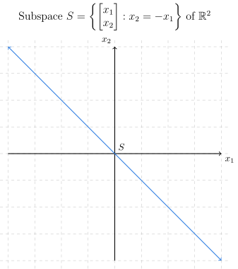
Let us show that subset $S$ is a subspace.
1. First we must show that the set is nonempty. Consider the zero vector $\mathbf{u} = \begin{bmatrix}\ 0\ \\ \ 0\ \end{bmatrix}$. Since $u_2 = 0 = -0 = -u_1$ we have that $\mathbf{u}\in S$, and $S\neq\emptyset$.
2. We need a way to represent elements of our nonempty set $S$. Since the second coordinate is always the negative of the first coordinate, we can use the notation
$$ \mathbf{a} = \begin{bmatrix}\ \ a\ \\ -a\ \end{bmatrix}\in S $$
for some number $a$, and multiply this by a scalar $t$.
$$ t\,\mathbf{a} = t\,\begin{bmatrix}\ \ a\ \\ -a\ \end{bmatrix} = \begin{bmatrix}\ \ ta\ \\ -ta\ \end{bmatrix}\in S $$
This shows that $S$ is closed under scalar multiplication.
3. For the closure of vector addition, we consider two elements of $S$
$$ \begin{bmatrix}\ \ a\ \\ -a\ \end{bmatrix} \qquad\text{and}\qquad \begin{bmatrix}\ \ b\ \\ -b\ \end{bmatrix} $$
The sum
$$ \begin{bmatrix}\ \ a\ \\ -a\ \end{bmatrix} + \begin{bmatrix}\ \ b\ \\ -b\ \end{bmatrix} = \begin{bmatrix}\ \ a + b\ \\ -a + (-b)\ \end{bmatrix} = \begin{bmatrix}\ \ a + b\ \\ -(a + b)\ \end{bmatrix}\in S $$
Since we have satisfied the closure properties, we say that $S$ is a subspace of $\mathbb{R}^2$, and that $S$ is itself a vector space.
Why do we need only show that the closure properties are satisfied?
The eight axioms of a vector space apply to every element of the vector space. In particular, they apply to all of the vectors in subset $S$.
The closure properties are qualities of the subset $S$, not a property of the vectors in it. The eight axioms are properties of the algebra of the vectors.
Proof of Theorem 1
Subspaces, by definition, are nonempty subsets $S$ of $V$ for which the closure properties hold. Since $S$ is nonempty let vector $\mathbf{x}\in S$. Since $S$ is closed under scalar multiplication, $-1\cdot\mathbf{x} = -\mathbf{x}\in S$. Since $S$ is closed under vector addition, $-\mathbf{x}+\mathbf{x} = \mathbf{0}\in S$. $\blacksquare$
Example 2 - Uninteresting Subspaces
Every vector space $V$ has two subspaces
$V$ is a subspace of $V$. You can check the definition. $V\subseteq V$, and it is closed under linear combinations.
$\left\{\mathbf{0}\right\}$ is a subspace of $V$. The sum of zero vectors is the zero vector. A scalar multiple of the zero vector is the zero vector. This subspace is called the trivial subspace.

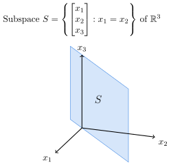
Example 3 - Plane in 3D-Space
1. Let the set $S$ be defined by
$$ S = \left\{ \begin{bmatrix}\ x_1\ \\ \ x_2\ \\ \ x_3\ \end{bmatrix} \in\mathbb{R}^3 : x_1 = x_2 \right\} $$
To verify this is a subspace, we check that it contains $\mathbf{0}$, which it does since
$$ \mathbf{0} = \begin{bmatrix}\ 0\ \\ \ 0\ \\ \ 0\ \end{bmatrix} \in S $$
Next, we need to see if it obeys the closure properties.
If $(a,a,b)^T\in S$, then for any scalar $t$ we have
$$ t\,(a,a,b)^T = (ta,ta,tb)^T \in S $$If $(a,a,b)^T,(c,c,d)^T\in S$, then
$$ (a,a,b)^T + (c,c,d)^T = (a+c,a+c,b+d)^T \in S $$
Therefore, $S$ is a subspace of $\mathbb{R}^3$. It is a plane through the origin.
Example 4 - A Line in 2D-Space
Let $S = \left\{ (x,1)^T : x\in\mathbb{R}\right\} $.
This is not a subspace of $\mathbb{R}^2$ for multiple reasons:
It does not contain $\mathbf{0}$, since there is no choice of $x$ where $(x,1)^T$ will be $(0,0)^T$. This will ultimately prevent the subset from satisfying Theorem 1. If every subspace contains the zero vector, any subset that does not contain the zero vector is not a subspace.
This subset is not closed under scalar multiplication $$ 3\,\begin{bmatrix}\ \ x\ \\ \ \ 1\ \end{bmatrix} = \begin{bmatrix}\ \ 3x\ \\ \ \ 3\ \end{bmatrix} \notin S $$
This subset is not closed under vector addition $$ \begin{bmatrix}\ \ x\ \\ \ \ 1\ \end{bmatrix} + \begin{bmatrix}\ \ y\ \\ \ \ 1\ \end{bmatrix} = \begin{bmatrix}\ x+y\ \\ \ 2\ \end{bmatrix} \notin S $$
Any one of these counterexamples shows that $S$ is not a subspace.

One need only show one of these properties is false for our set $S$ to show that it cannot be a subspace of $\mathbb{R}^2$.
Everyone viewed this video at the beginning of the semester. This is a good review. We should all see the ideas in this video with greater insight.
Video Lecture 2 - Span
 Span
SpanDefinition
Span
Let $\mathbf{v}_1,\mathbf{v}_2,\ldots,\mathbf{v}_k$ be a set of vectors in a vector space $V$. The set of all possible linear combinations $$\ t_1\mathbf{v}_1 + t_2\mathbf{v}_2 + \ldots + t_k\mathbf{v}_k$$ for scalars $t_j$, $1\le j\le k$ is called the span of $\mathbf{v}_1,\mathbf{v}_2,\ldots,\mathbf{v}_k$ and is denoted $\textrm{Span}\left(\mathbf{v}_1,\mathbf{v}_2,\ldots,\mathbf{v}_k\right)$.
The span of a set of vectors is the set of all vectors in a space that may be "reached" by computing a linear combination of the vectors in the set.
Example 5 - A Spanning Set of a Subspace
We can write down a set that spans the subspace from Example 3
$$ \begin{bmatrix}\ a\ \\ \ a\ \\ \ b\ \end{bmatrix} = a\begin{bmatrix}\ 1\ \\ \ 1\ \\ \ 0\ \end{bmatrix} + b\begin{bmatrix}\ 0\ \\ \ 0\ \\ \ 1\ \end{bmatrix} $$
A linear combination of these two vectors will generate a vector that reaches each point on the plane $S$ in the figure from that example.
$$ S = \textrm{Span}\left\{ \begin{bmatrix}\ 1\ \\ \ 1\ \\ \ 0\ \end{bmatrix},\ \begin{bmatrix}\ 0\ \\ \ 0\ \\ \ 1\ \end{bmatrix} \right\} $$
Since this subset $S$ is the span of two linearly independent vectors, it is a plane. Since it is a span of vectors it is a subspace.
We call sets like
$$ B = \left\{ \begin{bmatrix}\ 1\ \\ \ 1\ \\ \ 0\ \end{bmatrix},\ \begin{bmatrix}\ 0\ \\ \ 0\ \\ \ 1\ \end{bmatrix} \right\} $$
a spanning set because we found two vectors in subspace $S$ that span $S$. That is $S = \textrm{Span}(B)$.
Definition
Definition of Spanning Set
The set $\left\{\mathbf{v}_1,\mathbf{v}_2,\ldots,\mathbf{v}_k\right\}$ is a spanning set for $V$ if and only if every vector $\mathbf{v}\in V$ may be written as a linear combination of $\mathbf{v}_1,\mathbf{v}_2,\ldots,\mathbf{v}_k$.
Our task in future chapters will be to characterize properties of Subspaces by determining a spanning set for the Subspace. The vectors in a spanning set provide important information about the subspace.
Theorem 2
The Span of a Set of Vectors is a Subspace
If $\mathbf{v}_1,\mathbf{v}_2,\ldots,\mathbf{v}_k$ are vectors in a vector space $V$, then $\ \textrm{Span}\left(\mathbf{v}_1,\mathbf{v}_2,\ldots,\mathbf{v}_k\right)$ is a subspace of $V$.
Proof of Theorem 2
The set $S=\textrm{Span}\left(\mathbf{v}_1,\mathbf{v}_2,\ldots,\mathbf{v}_k\right)$ is nonempty, since $$\mathbf{0} = 0\mathbf{v}_1 + \cdots + 0\mathbf{v}_k \in S.$$
Let $c$ be a scalar and let $\mathbf{v} = t_1 \mathbf{v}_1 + t_2 \mathbf{v}_2 + \cdots + t_k \mathbf{v}_k$ be any vector in $\textrm{Span}\left(\mathbf{v}_1,\dots,\mathbf{v}_k\right)$. Then we have
$$ \begin{align*} c\mathbf{v} &= c\left(t_1 \mathbf{v}_1 + \cdots + t_k\mathbf{v}_k\right) \\ &= (ct_1)\mathbf{v}_1 + \cdots + (ct_k) \mathbf{v}_k\in S. \end{align*} $$
If we let $\mathbf{v} = t_1 \mathbf{v}_1 + \cdots + t_k \mathbf{v}_k$ and $\mathbf{w} = u_1 \mathbf{v}_1 + \cdots + u_k \mathbf{v}_k$ be any two vectors in the span, then
$$ \mathbf{v} + \mathbf{w} = (t_1 + u_1)\mathbf{v}_1 + \cdots + (t_k + u_k)\mathbf{v}_k\in S.$$
Hence, $\textrm{Span}\left(\mathbf{v}_1,\mathbf{v}_2,\ldots,\mathbf{v}_k\right)$ is a subspace of $V$. $\blacksquare$
Spanning sets are not unique. We will discover techniques for determining a spanning set for a subspace. We will develop techniques for choosing a spanning set with convenient properties.
Example 6 - Spanning Sets of a Subspace
Both the sets span $\mathbb{R}^2$.
$$C = \left\{\,\mathbf{e}_1,\ \mathbf{e}_2\,\right\} = \left\{\, \begin{bmatrix}\ 1\ \\ \ 0\ \end{bmatrix},\ \begin{bmatrix}\ 0\ \\ \ 1\ \end{bmatrix} \,\right\}$$
and
$$B = \left\{\, \mathbf{v}_1,\ \mathbf{v}_2 \,\right\} = \left\{ \begin{bmatrix}\ 1\ \\ \ 1\ \end{bmatrix},\ \begin{bmatrix}\ 0\ \\ \ 1\ \end{bmatrix} \,\right\}$$
It is always possible to write any vector in $\mathbb{R}^2$ as a linear combination of either $\left\{\mathbf{e}_1,\mathbf{e}_2\right\}$ or $\left\{\mathbf{v}_1,\mathbf{v}_2\right\}$.
Let $\langle a, b \rangle$ be any vector in $\mathbb{R}^2$. We will demonstrate that it is possible to always write this vector as a linear combination of either of the proposed spanning sets. For set $C = \left\{\mathbf{e}_1,\mathbf{e}_2\right\}$, this is easy.
$$ \begin{bmatrix}\ a\ \\ \ b\ \end{bmatrix} = a \begin{bmatrix}\ 1\ \\ \ 0\ \end{bmatrix} + b \begin{bmatrix}\ 0\ \\ \ 1\ \end{bmatrix} = \begin{bmatrix}\ 1\ &\ 0\ \\ \ 0\ &\ 1\ \end{bmatrix}\begin{bmatrix}\ a\ \\ \ b\ \end{bmatrix} $$
For $\left\{\mathbf{v}_1,\mathbf{v}_2\right\}$, we have
$$ \begin{bmatrix}\ a\ \\ \ b\ \end{bmatrix} = x_1 \begin{bmatrix}\ 1\ \\ \ 1\ \end{bmatrix} + x_2 \begin{bmatrix}\ 0\ \\ \ 1\ \end{bmatrix} = \begin{bmatrix}\ 1\ &\ 0\ \\ \ 1\ &\ 1\ \end{bmatrix}\begin{bmatrix}\ x_1\ \\ \ x_2\ \end{bmatrix} $$
and we need to show that the associated linear system
$$ \begin{align*} x_1 &= a \\ x_1 + x_2 &= b \end{align*} $$
is consistent.
$$ \left[ \begin{array}{cc|c}\ 1\ &\ 0 &\ a\ \\ \ 1\ &\ 1 &\ b\ \end{array} \right]\begin{array}{l} \\ R_2-R_1 \end{array} \rightarrow \left[ \begin{array}{cc|c}\ 1\ &\ 0 &\ a\ \\ \ 0\ &\ 1 & b-a \end{array} \right] $$
Both columns are pivot columns so the matrix $\begin{bmatrix}\ 1\ &\ 0\ \\ \ 1\ &\ 1 \ \end{bmatrix}$ is nonsingular. The solution to the linear system is the vector $\begin{bmatrix}\ a\ \\ b-a \end{bmatrix}$. We can conclude that the solution is unique because the matrix is nonsingular.
We have shown that every vector $\begin{bmatrix}\ a\ \\ \ b\ \end{bmatrix}\in\mathbb{R}^2$ can be written as a linear combination of $\mathbf{v}_1$ and $\mathbf{v}_2$. Hence we say that the set $B = \left\{\mathbf{v}_1,\mathbf{v}_2\right\}$ spans $\mathbb{R}^2$.
Exercise 1 - Spanning Set of $\mathbb{R}^3$
Determine if
$$B = \left\{\ \begin{bmatrix} -1\ \\ \ 2\ \\ \ 1\ \end{bmatrix},\ \begin{bmatrix}\ 0\ \\ \ 3\ \\ -1\ \end{bmatrix},\ \begin{bmatrix}\ 2\ \\ -1\ \\ -3\ \end{bmatrix}\ \right\}$$
spans $\mathbb{R}^3$.
Follow Along
For set $B$ to span $\mathbb{R}^3$, we need to be able to express an arbitrary point $\langle a,b,c \rangle$ in $\mathbb{R}^3$ as a linear combination of the vectors in set $B$. $$ \begin{bmatrix}\ a\ \\ \ b\ \\ \ c\ \end{bmatrix} = x_1 \begin{bmatrix} -1\ \\ \ 2\ \\ \ 1\ \end{bmatrix} + x_2 \begin{bmatrix}\ 0\ \\ \ 3\ \\ -1\ \end{bmatrix} + x_3 \begin{bmatrix}\ 2\ \\ -1\ \\ -3\ \end{bmatrix} $$ This corresponds to the linear system $$ \begin{array}{rcr} -x_1 \, \ \ \ \ \ \ \ \ \ \ + 2x_3 & = & a \\ 2x_1 + 3x_2 - 1x_3 & = & b \\ \ \ x_1 - 1x_2 - 3x_3 & = & c \end{array} $$ whose coefficient matrix is given by $$ \begin{align*} \begin{bmatrix} -1\ &\ 0\ &\ 2\ \\ \ 2\ &\ 3\ & -1\ \\ \ 1\ & -1\ & -3\ \end{bmatrix}\begin{array}{r} \\ R_2+2R_1 \\ R_3+R_1 \end{array} &\rightarrow \begin{bmatrix} -1\ &\ 0\ &\ 2\ \\ \ 0\ &\ 3\ &\ \ 3\ \\ \ 0\ & -1\ & -1\ \end{bmatrix}\begin{array}{r} -R_1 \\ R_2/3 \\ \\ \end{array} \rightarrow \\ \\ \begin{bmatrix}\ 1\ &\ 0\ & -2\ \\ \ 0\ &\ 1\ &\ \ 1\ \\ \ 0\ & -1\ & -1\ \end{bmatrix}\begin{array}{r} \\ \\ R_3+R_2 \end{array} &\rightarrow \begin{bmatrix}\ 1\ &\ 0\ & -2\ \\ \ 0\ &\ 1\ &\ \ 1\ \\ \ 0\ &\ 0\ &\ 0\ \end{bmatrix} \end{align*} $$ This implies that the system is singular, since the coefficient matrix is a $3\times 3$ matrix with only two pivot columns. Because the system is singular, it cannot be solved for all vectors $(a,b,c)^T\in\mathbb{R}^3$. Our set does not span $\mathbb{R}^3$.One may also conclude that the span of the columns of coefficient matrix is a plane since it has only two pivot columns. Thus it cannot be all of $\mathbb{R}^3$.
This problem could have been solved using inspection by seeing how to write the third column vector in our set as a linear combination of the first two. The coefficients for this are revealed by the above reduced row echelon form.
$$ \begin{bmatrix}\ 1\ &\ 0\ & \color{#9900FF}{-2}\ \\ \ 0\ &\ 1\ &\ \color{#CC0099}{1}\ \\ \ 0\ &\ 0\ &\ 0\ \end{bmatrix} $$
$$ \begin{bmatrix}\ 2\ \\ -1\ \\ -3\ \end{bmatrix} = \color{#9900FF}{-2} \begin{bmatrix} -1\ \\ \ 2\ \\ \ 1\ \end{bmatrix} + \color{#CC0099}{1}\begin{bmatrix}\ 0\ \\ \ 3\ \\ -1\ \end{bmatrix} $$ This means that the span of these three vectors $$ \left\{\ \begin{bmatrix} -1\ \\ \ 2\ \\ \ 1\ \end{bmatrix},\ \begin{bmatrix}\ 0\ \\ \ 3\ \\ -1\ \end{bmatrix},\ \begin{bmatrix}\ 2\ \\ -1\ \\ -3\ \end{bmatrix}\ \right\} $$ is only a plane because it only has two linearly independent vectors and one dependent vector.
Let us consider a linear transformation $L\,:\,\mathbb{R}^n\rightarrow\mathbb{R}^m$ defined by $$L(\mathbf{x}) = A\mathbf{x}$$ for $m\times n$ matrix $A$. Recall that the columns of matrix $A$ are the images of the basis vectors of $\mathbb{R}^n$ in $\mathbb{R}^m$. In standard coordinates we have the standard basis vectors $\mathbf{e}_1$, $\dots$, $\mathbf{e}_n$. These special vectors have a familiar pattern to them in our standard coordinate system.
In $\mathbb{R}^2$, we have
$$ \mathbf{e}_1 = \ihat = \begin{bmatrix}\ 1\ \\ \ 0\ \end{bmatrix},\ \text{ and }\ \mathbf{e}_2 = \jhat = \begin{bmatrix}\ 0\ \\ \ 1\ \end{bmatrix} $$
In $\mathbb{R}^3$, we have
$$ \mathbf{e}_1 = \ihat = \begin{bmatrix}\ 1\ \\ \ 0\ \\ \ 0\ \end{bmatrix},\ \mathbf{e}_2 = \jhat = \begin{bmatrix}\ 0\ \\ \ 1\ \\ \ 0\ \end{bmatrix},\ \text{and}\ \mathbf{e}_3 = \khat = \begin{bmatrix}\ 0\ \\ \ 0\ \\ \ 1\ \end{bmatrix} $$
In $\mathbb{R}^n$, we have
$$ \mathbf{e}_1 = \begin{bmatrix}\ 1\ \\ \ 0\ \\ \ \vdots\ \\ \ 0\ \end{bmatrix},\ \mathbf{e}_2 = \begin{bmatrix}\ 0\ \\ \ 1\ \\ \ \vdots\ \\ \ 0\ \end{bmatrix},\ \dots,\ \text{and}\ \mathbf{e}_n = \begin{bmatrix}\ 0\ \\ \ \vdots\ \\ \ 0\ \\ \ 1\ \end{bmatrix} $$
Remember $A\mathbf{e}_k$ is the $k^{\text{th}}$ column of matrix $A$. The coordinates of this column of matrix $A$ are the coordinates of vector $L(\mathbf{e}_k) = A\mathbf{e}_k = \mathbf{a}_k$ in $\mathbb{R}^m$. This is the image of vector $\mathbf{e}_k$ under the linear transformation, as well as the column $\mathbf{a}_k$ of matrix $A$.
Any vector in $\mathbf{x}\in\mathbb{R}^n$ can be written as a linear combination of our standard basis vectors,
$$ \mathbf{x} = \begin{bmatrix}\ x_1\ \\ \ x_2\ \\ \vdots\ \\ \ x_n\ \end{bmatrix} = x_1\mathbf{e}_1 + x_2\mathbf{e}_2 + \dots + x_n\mathbf{e}_n $$
The image of every vector $\mathbf{x}\in\mathbb{R}^n$ is the same linear combination of the columns of matrix $A$.
$$ \begin{align*} A\mathbf{x} &= A\left(x_1\mathbf{e}_1 + x_2\mathbf{e}_2 + \dots + x_n\mathbf{e}_n\right) \\ \\ &= x_1A\mathbf{e}_1 + x_2A\mathbf{e}_2 + \dots + x_nA\mathbf{e}_n \\ \\ &= x_1\mathbf{a}_1 + x_2\mathbf{a}_2 + \dots + x_n\mathbf{a}_n \end{align*} $$
Notice that the elements of vector $\mathbf{x}$ are the coefficients of the standard basis vectors in the domain $\mathbb{R}^n$, and the coefficients of the columns of matrix $A$ in $\mathbb{R}^m$. Now we can ask ourselves an interesting question,
$$ \textbf{What is the set of all image vectors in $\mathbf{\mathbb{R}^m}$?} $$
This would be the set of possible linear combinations of the columns of matrix $A$, or span of the column vectors of matrix $A$ in $\mathbb{R}^m$. This subspace of the codomain is called the column space of matrix $A$.
Definition
Column Space
The column space $C(A)$ of an $m\times n$ matrix $A$ is the span of the column vectors in matrix $A$. $C(A)$ is a subspace of $\mathbb{R}^m$.
$$ \begin{align*} C(A) &:= \left\{ A\mathbf{x}:\,\mathbf{x}\in\mathbb{R}^n \right\}\subseteq\mathbb{R}^m \\ \\ &= \left\{ x_1\mathbf{a}_1 + x_2\mathbf{a}_2 + \dots + x_n\mathbf{a}_n\,:\,(x_1,x_2,\dots,x_n)^T\in\mathbb{R}^n\right\} \end{align*} $$
Exercise 2 - Determine the Column Space of Each Matrix
The column space $C(A)$ is the span of the columns of $A$, a subspace of the codomain $\mathbb{R}^3$. Row reduce each matrix to locate the pivot columns; the corresponding columns of the original matrix form a basis for $C(A)$. Determine the column space of each of the following matrices.
$$ A = \begin{bmatrix}\ 1\ &\ 0\ &\ 2\ \\ \ 2\ &\ 1\ &\ 3\ \\ \ 1\ &\ 1\ &\ 2\ \end{bmatrix} \qquad B = \begin{bmatrix}\ 1\ &\ 2\ &\ 3\ \\ \ 0\ &\ 1\ &\ 1\ \\ \ 2\ &\ 1\ &\ 3\ \end{bmatrix} \qquad C = \begin{bmatrix}\ 1\ &\ 2\ & -1\ \\ \ 2\ &\ 4\ & -2\ \\ -1\ & -2\ &\ 1\ \end{bmatrix} $$
Follow Along — Matrix $A$
Row reduce $A$.$$ \begin{bmatrix}\ 1\ &\ 0\ &\ 2\ \\ \ 2\ &\ 1\ &\ 3\ \\ \ 1\ &\ 1\ &\ 2\ \end{bmatrix} \begin{array}{r} \\ R_2-2R_1 \\ R_3-R_1 \end{array} \rightarrow \begin{bmatrix}\ 1\ &\ 0\ &\ 2\ \\ \ 0\ &\ 1\ & -1\ \\ \ 0\ &\ 1\ &\ 0\ \end{bmatrix} \begin{array}{r} \\ \\ R_3-R_2 \end{array} \rightarrow \begin{bmatrix}\ 1\ &\ 0\ &\ 2\ \\ \ 0\ &\ 1\ & -1\ \\ \ 0\ &\ 0\ &\ 1\ \end{bmatrix} $$
All three columns are pivot columns, so the columns of $A$ are linearly independent and $$ C(A) = \mathbb{R}^3. $$
Follow Along — Matrix $B$
Row reduce $B$.$$ \begin{bmatrix}\ 1\ &\ 2\ &\ 3\ \\ \ 0\ &\ 1\ &\ 1\ \\ \ 2\ &\ 1\ &\ 3\ \end{bmatrix} \begin{array}{r} \\ \\ R_3-2R_1 \end{array} \rightarrow \begin{bmatrix}\ 1\ &\ 2\ &\ 3\ \\ \ 0\ &\ 1\ &\ 1\ \\ \ 0\ & -3\ & -3\ \end{bmatrix} \begin{array}{r} R_1-2R_2 \\ \\ R_3+3R_2 \end{array} \rightarrow \begin{bmatrix}\ 1\ &\ 0\ &\ 1\ \\ \ 0\ &\ 1\ &\ 1\ \\ \ 0\ &\ 0\ &\ 0\ \end{bmatrix} $$
The pivots are in columns 1 and 2, so a basis for the column space is $$ C(B) = \textrm{Span}\left\{ \begin{bmatrix}\ 1\ \\ \ 0\ \\ \ 2\ \end{bmatrix},\ \begin{bmatrix}\ 2\ \\ \ 1\ \\ \ 1\ \end{bmatrix} \right\}. $$ The reduced form shows the third column is the sum of the first two, $\mathbf{b}_3 = \mathbf{b}_1 + \mathbf{b}_2$, so it contributes nothing new. The column space is a plane through the origin, with equation $-2x + 3y + z = 0$.
Follow Along — Matrix $C$
Row reduce $C$.$$ \begin{bmatrix}\ 1\ &\ 2\ & -1\ \\ \ 2\ &\ 4\ & -2\ \\ -1\ & -2\ &\ 1\ \end{bmatrix} \begin{array}{r} \\ R_2-2R_1 \\ R_3+R_1 \end{array} \rightarrow \begin{bmatrix}\ 1\ &\ 2\ & -1\ \\ \ 0\ &\ 0\ &\ 0\ \\ \ 0\ &\ 0\ &\ 0\ \end{bmatrix} $$
Only the first column is a pivot column. Every column is a multiple of the first ($\mathbf{c}_2 = 2\mathbf{c}_1$, $\mathbf{c}_3 = -\mathbf{c}_1$), so $$ C(C) = \textrm{Span}\left\{ \begin{bmatrix}\ 1\ \\ \ 2\ \\ -1\ \end{bmatrix} \right\}, $$ a line through the origin.
The column space of a matrix tells us important information about linear system $A\mathbf{x}=\mathbf{b}$.
Theorem 3
Consistency Check
The linear system $A\mathbf{x}=\mathbf{b}$ is consistent if and only if $\mathbf{b}\in C(A)$.
Proof of Theorem 3
As with our previous if and only if theorems, we must show both that
The linear system $A\mathbf{x}=\mathbf{b}$ is consistent $\implies$ $\mathbf{b}\in C(A)$
$\mathbf{b}\in C(A)\ \implies$ the linear system $A\mathbf{x}=\mathbf{b}$ is consistent.
$\left(\Rightarrow\right)$ If the linear system $A\mathbf{x}=\mathbf{b}$ is consistent, then there is at least one vector $\mathbf{x}_0\in\mathbb{R}^n$ so that $A\mathbf{x}_0=\mathbf{b}$. As $C(A) = \left\{ A\mathbf{x}\,:\,\mathbf{x}\in\mathbb{R}^n\right\}$, we have that $\mathbf{b}=A\mathbf{x}_0\in C(A)$.
$\left(\Leftarrow\right)$ If $\mathbf{b}\in C(A)$, then $\mathbf{b}\in\left\{ A\mathbf{x}\,:\,\mathbf{x}\in\mathbb{R}^n\right\}$. So there must be at least one vector $\mathbf{x}_0$ so that $\mathbf{b}=A\mathbf{x}_0$. Thus the linear system $A\mathbf{x}=\mathbf{b}$ has at least one solution and it is consistent. $\blacksquare$
Exercise 3 - Determine whether each Linear System is Consistent
Using the matrices defined in exercise 2, determine whether each of the following linear systems are consistent.
$$ A\mathbf{x} = \begin{bmatrix}\ \ 3\ \\ \ \ 4\ \\ -4\ \end{bmatrix} \qquad B\mathbf{x} = \begin{bmatrix}\ 0\ \\ \ 0\ \\ \ 1\ \end{bmatrix} \qquad C\mathbf{x} = \begin{bmatrix}\ 6\ \\ 12\ \\ -6\ \end{bmatrix} $$
Follow Along — Matrix $A$
All of the columns of matrix $A$ are pivot columns. Thus matrix $A$ is non-singular. $A\mathbf{x}=\mathbf{b}$ is consistent for any $\mathbf{b}\in\mathbb{R}^3$. So it is consistent for $\mathbf{b} = \langle 3, 4, -4 \rangle$.Follow Along — Matrix $B$
The first two columns of matrix $B$ are the pivot columns. For $B\mathbf{x}=\mathbf{b}$ to be consistent, $\mathbf{b}$ must be a vector in $$\textrm{Span}\left\{\,\begin{bmatrix}\ 1\ \\ \ 0\ \\ \ 2\ \end{bmatrix},\ \begin{bmatrix}\ 2\ \\ \ 1\ \\ \ 1\ \end{bmatrix}\,\right\}$$ We must solve $$\begin{align*} \left[ \begin{array}{cc|c}\ 1\ &\ 2\ &\ 0\ \\ \ 0\ &\ 1\ &\ 0\ \\ \ 2\ &\ 1\ &\ 1\ \end{array} \right]\begin{array}{r} \\ \\ R_3-2R_1 \end{array} &\rightarrow \left[ \begin{array}{cc|c}\ 1\ &\ 2\ &\ 0\ \\ \ 0\ &\ 1\ &\ 0\ \\ \ 0\ & -3\ &\ 1\ \end{array} \right]\begin{array}{r} \\ \\ R_3+3R_2 \end{array} \rightarrow \left[ \begin{array}{cc|c}\ 1\ &\ 2\ &\ 0\ \\ \ 0\ &\ 1\ &\ 0\ \\ \ 0\ &\ 0\ &\ 1\ \end{array} \right] \end{align*}$$ This linear system is inconsistent; $\mathbf{b}$ is *not* a linear combination of the pivot columns of matrix $B$; $\mathbf{b}\notin C(B)$. Hence the linear system is inconsistent for $\mathbf{b} = \langle 0, 0, 1 \rangle$.Follow Along — Matrix $C$
Matrix $C$ has one pivot column $\langle 1, 2, -1 \rangle$. Furthermore, $\mathbf{b} = \langle 6, 12, -6 \rangle = 6\langle 1, 2, -1 \rangle$ implies that $$\mathbf{b}\in C(C) = \textrm{Span}\left\{\, \begin{bmatrix}\ \ 1\ \\ \ \ 2\ \\ -1\ \end{bmatrix} \,\right\}$$ Hence the linear system $C\mathbf{x} = \langle 6, 12, -6 \rangle$ is consistent.The column space of a matrix is a subspace of the codomain. The Null Space of a matrix is a subspace of the domain. Consider $m\times n$ matrix $A$ and the solution set of the homogeneous equation
$$ A\mathbf{x} = \mathbf{0} $$
Let us define the solution set $N(A) = \left\{\,\mathbf{x}\in\mathbb{R}^n \,:\, A\mathbf{x}=\mathbf{0} \,\right\}$.
We know that $N(A)$ is nonempty because the zero vector $\mathbf{0}\in N(A)$.
If $\mathbf{x}_1$ and $\mathbf{x}_2\in N(A)$, then $A(\mathbf{x}_1 + \mathbf{x}_2) = A\mathbf{x}_1 + A\mathbf{x}_2 = \mathbf{0} + \mathbf{0} = \mathbf{0}$. Thus $\mathbf{x}_1+\mathbf{x}_2\in N(A)$.
If $\mathbf{x}\in N(A)$ and $c$ is a scalar, then $A(c\mathbf{x}) = cA\mathbf{x} = c\mathbf{0} = \mathbf{0}$. Thus $c\mathbf{x}\in N(A)$.
Definition
The Null Space $N(A)$ of an $m\times n$ matrix $A$ is the set of vectors in $\mathbb{R}^n$ defined by
$$ N(A) = \left\{ \mathbf{x}\in\mathbb{R}^n\,:\,A\mathbf{x}=\mathbf{0}\right\} $$
The column space of a matrix $C(A)$ is defined to be the span of the column vectors of the matrix and we already know that it is a subspace of $\mathbb{R}^m$ because it is a span or all possible linear combinations of the columns of matrix $A$.
However, the null space is to be the set of all possible solutions to $A\mathbf{x}=\mathbf{0}$. This is not immediately a subspace. We are obligated to show that $N(A)$ is indeed a subspace of $\mathbb{R}^n$.
Theorem 4
Null Space
The null space $N(A)$ of $m\times n$ matrix $A$ is a subspace of $\mathbb{R}^n$.
Proof of Theorem 4
Items 1.-3., before the definition of null space, show that the null space of a matrix is closed under linear combinations. $\blacksquare$
Example 7 - Determine the Null Space
Determine the null space $N(A)$ if
$$ A = \begin{bmatrix}\ 1\ &\ 2\ & -3\ & -1\ \\ -2\ & -4\ &\ 6\ &\ 3\ \end{bmatrix} $$
We begin by writing the augmented matrix that represents the homogeneous equation $A\mathbf{x} = \mathbf{0}$
$$ \left[ \begin{array}{cccc|c}\ 1\ &\ 2\ & -3\ & -1 & 0\ \\ -2\ & -4\ &\ 6\ &\ 3 & 0\ \end{array} \right]$$
The augmented matrix is not really necessary as the right-hand side will always be zeros. Performing necessary elementary row operations in order to reduce matrix $A$ to reduced row echelon form:
$$ \begin{align*} \begin{bmatrix}\ 1\ &\ 2\ & -3\ & -1\ \\ -2\ & -4\ &\ 6\ &\ 3\ \end{bmatrix}\begin{array}{c} \ \\ R_2 + 2R_1 \end{array} &\rightarrow \begin{bmatrix}\ 1\ &\ 2\ & -3\ & -1\ \\ \ 0\ &\ 0\ &\ 0\ &\ 1\ \end{bmatrix}\begin{array}{c} \ R_1+R_2 \\ \ \end{array} \\ \\ &\rightarrow \begin{bmatrix}\ 1\ &\ 2\ & -3\ &\ 0\ \\ \ 0\ &\ 0\ &\ 0\ &\ 1\ \end{bmatrix} \end{align*} $$
We see from reduced row echelon form that we have two free variables $x_2$ and $x_3$
$$ \begin{align*} x_2 &= \alpha\in\mathbb{R} \\ x_3 &= \beta\in\mathbb{R} \\ x_4 &= 0 \\ x_1 + 2\alpha - 3\beta &= 0 \\ x_1 &= -2\alpha + 3\beta \end{align*} $$
$$ \mathbf{x} = \begin{bmatrix} -2\alpha + 3\beta \\ \alpha \\ \beta \\ 0 \end{bmatrix} = \alpha \begin{bmatrix} -2\ \\ \ \ 1\ \\ \ \ 0\ \\ \ \ 0\ \end{bmatrix} + \beta \begin{bmatrix}\ \ 3\ \\ \ \ 0\ \\ \ \ 1\ \\ \ \ 0\ \end{bmatrix} $$
are solutions of $A\mathbf{x} = \mathbf{0}$. Hence, $N(A)$ is composed of all vectors of the form
$$ \alpha \begin{bmatrix} -2\ \\ \ \ 1\ \\ \ \ 0\ \\ \ \ 0\ \end{bmatrix} + \beta \begin{bmatrix}\ 3\ \\ \ 0\ \\ \ 1\ \\ \ 0\ \end{bmatrix} $$
We can say that the null space of this matrix is a span of vectors
$$ N(A) = \textrm{Span}\left\{ \begin{bmatrix} -2\ \\ \ \ 1\ \\ \ \ 0\ \\ \ \ 0\ \end{bmatrix},\ \begin{bmatrix}\ 3\ \\ \ 0\ \\ \ 1\ \\ \ 0\ \end{bmatrix} \right\} $$
The null space of a matrix tells us important information about the number of solutions of any consistent linear system $A\mathbf{x} = \mathbf{b}$.
Theorem 5
The solution of a consistent nonhomogeneous linear system of equations
$$ A\mathbf{x} = \mathbf{b} $$
is unique if and only if the null space of $A$ is trivial, that is
$$ N(A) = \left\{\mathbf{0}\right\} $$
Proof of Theorem 5
To prove this, we need to show both
- A trivial null space $\implies$ that a solution to consistent linear system $A\mathbf{x}=\mathbf{b}$ is unique.
- If consistent linear systems $A\mathbf{x}=\mathbf{b}$ has a unique solution, then $N(A)$ is trivial.
$\left(\Rightarrow\right)$ First, suppose that $N(A)$ is trivial and the consistent linear system has solutions $A\mathbf{x} = \mathbf{b}$ and $A\mathbf{y} = \mathbf{b}$. Then
$$ \begin{align*} A\mathbf{x} - A\mathbf{y} &= \mathbf{b} - \mathbf{b} \\ A(\mathbf{x} - \mathbf{y}) &= \mathbf{0} \end{align*} $$
Since $N(A)$ is trivial, it must be the case that
$$ \begin{align*} \mathbf{x} - \mathbf{y} &= \mathbf{0} \\ \mathbf{x} &= \mathbf{y} \end{align*} $$
The solution to the consistent linear system is unique.
$\left(\Leftarrow\right)$ Now, suppose the solution to consistent linear system $A\mathbf{x} = \mathbf{b}$ is unique. Let $\mathbf{y}$ be an element of the null space $N(A)$, so $A\mathbf{y} = \mathbf{0}$. Then we have
$$ \begin{align*} A\mathbf{x} + A\mathbf{y} &= \mathbf{b} + \mathbf{0} \\ A(\mathbf{x} + \mathbf{y}) &= \mathbf{b} \end{align*} $$
This says that $\mathbf{x} + \mathbf{y}$ is a solution to the system $A\mathbf{x} = \mathbf{b}$, but we assumed that $\mathbf{x}$ is unique. Thus
$$ \begin{align*} \mathbf{x} + \mathbf{y} &= \mathbf{x} \\ \mathbf{y} &= \mathbf{0} \end{align*} $$
Since every element of the null space is $\mathbf{0}$, it must be that $\mathbf{0}$ is the only element of the null space. $N(A)$ is trivial. $\blacksquare$
Exercise 4 - Determine the Null Space of Each Matrix
Determine the null space $N(A)$, $N(B)$, and $N(C)$ for each of the following matrices.
$$ A = \begin{bmatrix}\ 1\ &\ 1\ &\ 1\ \\ \ 1\ &\ 2\ &\ 3\ \\ \ 1\ &\ 3\ &\ 6\ \\ \ 0\ &\ 1\ &\ 2\ \end{bmatrix} \qquad B = \begin{bmatrix}\ 1\ &\ 0\ &\ 0\ &\ 2\ \\ \ 1\ &\ 1\ &\ 0\ &\ 1\ \\ \ 0\ &\ 1\ &\ 1\ &\ 2\ \end{bmatrix} \qquad C = \begin{bmatrix}\ 1\ &\ 0\ &\ 2\ & -1\ \\ \ 1\ &\ 1\ &\ 3\ &\ 2\ \\ \ 2\ &\ 1\ &\ 5\ &\ 1\ \\ \ 1\ & -1\ &\ 1\ & -4\ \end{bmatrix} $$
Follow Along — Matrix $A$
Row reduce $A$.$$ \begin{bmatrix}\ 1\ &\ 1\ &\ 1\ \\ \ 1\ &\ 2\ &\ 3\ \\ \ 1\ &\ 3\ &\ 6\ \\ \ 0\ &\ 1\ &\ 2\ \end{bmatrix} \begin{array}{r} \\ R_2-R_1 \\ R_3-R_1 \\ \\ \end{array} \rightarrow \begin{bmatrix}\ 1\ &\ 1\ &\ 1\ \\ \ 0\ &\ 1\ &\ 2\ \\ \ 0\ &\ 2\ &\ 5\ \\ \ 0\ &\ 1\ &\ 2\ \end{bmatrix} \begin{array}{r} \\ \\ R_3-2R_2 \\ R_4-R_2 \end{array} \rightarrow \begin{bmatrix}\ 1\ &\ 1\ &\ 1\ \\ \ 0\ &\ 1\ &\ 2\ \\ \ 0\ &\ 0\ &\ 1\ \\ \ 0\ &\ 0\ &\ 0\ \end{bmatrix} $$
All three columns are pivot columns, so $A\mathbf{x}=\mathbf{0}$ has only the trivial solution. The null space is trivial, $$ N(A) = \left\{\mathbf{0}\right\}. $$ By Theorem 5, any consistent system $A\mathbf{x}=\mathbf{b}$ therefore has a unique solution.
Follow Along — Matrix $B$
Row reduce $B$.$$ \begin{bmatrix}\ 1\ &\ 0\ &\ 0\ &\ 2\ \\ \ 1\ &\ 1\ &\ 0\ &\ 1\ \\ \ 0\ &\ 1\ &\ 1\ &\ 2\ \end{bmatrix} \begin{array}{r} \\ R_2-R_1 \\ \\ \end{array} \rightarrow \begin{bmatrix}\ 1\ &\ 0\ &\ 0\ &\ 2\ \\ \ 0\ &\ 1\ &\ 0\ & -1\ \\ \ 0\ &\ 1\ &\ 1\ &\ 2\ \end{bmatrix} \begin{array}{r} \\ \\ R_3-R_2 \end{array} \rightarrow \begin{bmatrix}\ 1\ &\ 0\ &\ 0\ &\ 2\ \\ \ 0\ &\ 1\ &\ 0\ & -1\ \\ \ 0\ &\ 0\ &\ 1\ &\ 3\ \end{bmatrix} $$
The pivots are in columns 1, 2, and 3, so $x_4$ is the only free variable. Setting $x_4 = t$, $$ x_1 = -2t,\quad x_2 = t,\quad x_3 = -3t,\quad x_4 = t. $$ The null space is a line through the origin, $$ N(B) = \textrm{Span}\left\{ \begin{bmatrix} -2\ \\ \ \ 1\ \\ -3\ \\ \ \ 1\ \end{bmatrix} \right\}. $$
Follow Along — Matrix $C$
Row reduce $C$.$$ \begin{bmatrix}\ 1\ &\ 0\ &\ 2\ & -1\ \\ \ 1\ &\ 1\ &\ 3\ &\ 2\ \\ \ 2\ &\ 1\ &\ 5\ &\ 1\ \\ \ 1\ & -1\ &\ 1\ & -4\ \end{bmatrix} \begin{array}{r} \\ R_2-R_1 \\ R_3-2R_1 \\ R_4-R_1 \end{array} \rightarrow \begin{bmatrix}\ 1\ &\ 0\ &\ 2\ & -1\ \\ \ 0\ &\ 1\ &\ 1\ &\ 3\ \\ \ 0\ &\ 1\ &\ 1\ &\ 3\ \\ \ 0\ & -1\ & -1\ & -3\ \end{bmatrix} \begin{array}{r} \\ \\ R_3-R_2 \\ R_4+R_2 \end{array} \rightarrow \begin{bmatrix}\ 1\ &\ 0\ &\ 2\ & -1\ \\ \ 0\ &\ 1\ &\ 1\ &\ 3\ \\ \ 0\ &\ 0\ &\ 0\ &\ 0\ \\ \ 0\ &\ 0\ &\ 0\ &\ 0\ \end{bmatrix} $$
The pivots are in columns 1 and 2, so $x_3$ and $x_4$ are free. Setting $x_3 = s$ and $x_4 = t$, $$ x_1 = -2s + t,\quad x_2 = -s - 3t. $$ The null space is a plane through the origin, $$ N(C) = \textrm{Span}\left\{ \begin{bmatrix} -2\ \\ -1\ \\ \ \ 1\ \\ \ \ 0\ \end{bmatrix},\ \begin{bmatrix}\ \ 1\ \\ -3\ \\ \ \ 0\ \\ \ \ 1\ \end{bmatrix} \right\}. $$
Finally we are in a position to review solving $A\mathbf{x}=\mathbf{b}$ using the column space and the null space. This helps us understand when a solution exists, and when there are infinitely many solutions.
Video Lecture 3 - Solving Linear Systems.
Solving Linear SystemsExample 8 - Find the Complete Solution
Determine the complete solution to $A\mathbf{x}=\mathbf{b}$ where, $$A = \begin{bmatrix}\ \ 3\ &\ \ 0\ &\ \ 3\ & -3\ \\ \ \ 1\ &\ \ 3\ &\ \ 3\ & -1\ \\ -3\ &\ \ 3\ &\ \ 0\ &\ \ 3\ \\ -2\ & -2\ &\ \ 2\ &\ \ 2\ \end{bmatrix}\qquad \mathbf{b} = \begin{bmatrix} -9\ \\ -8\ \\ \ \ 0\ \\ -12\ \end{bmatrix}$$
1. Reduce the augmented matrix to reduced row echelon form (row echelon form or upper triangular form will also work, but reduced row echelon form is the most efficient).
$$ \begin{align*} \left[ \begin{array}{cccc|c}\ \ 3\ &\ \ 0\ &\ \ 3\ & -3\ & -9\ \\ \ \ 1\ &\ \ 3\ &\ \ 3\ & -1\ & -8\ \\ -3\ &\ \ 3\ &\ \ 0\ &\ \ 3\ &\ \ 0\ \\ -2\ & -2\ &\ \ 2\ &\ \ 2\ & -12\ \end{array} \right]\begin{array}{r} R_1/3 \\ \\ R_3/(-3) \\ R_4/(-2) \end{array} &\rightarrow \left[ \begin{array}{cccc|c}\ \ 1\ &\ \ 0\ &\ \ 1\ & -1\ & -3\ \\ \ \ 1\ &\ \ 3\ &\ \ 3\ & -1\ & -8\ \\ \ \ 1\ & -1\ &\ \ 0\ & -1\ &\ \ 0\ \\ \ \ 1\ &\ \ 1\ & -1\ & -1\ &\ \ 6\ \end{array} \right]\begin{array}{r} \\ R_2-R_1 \\ R_3-R_1 \\ R_4-R_1 \end{array} \rightarrow \\ \\ \left[ \begin{array}{cccc|c}\ \ 1\ &\ \ 0\ &\ \ 1\ & -1\ & -3\ \\ \ \ 0\ &\ \ 3\ &\ \ 2\ &\ \ 0\ & -5\ \\ \ \ 0\ & -1\ & -1\ &\ \ 0\ &\ \ 3\ \\ \ \ 0\ &\ \ 1\ & -2\ &\ \ 0\ &\ \ 9\ \end{array} \right]\begin{array}{r} \\ -R_3 \\ R_2 \\ \\ \end{array} &\rightarrow \left[ \begin{array}{cccc|c}\ \ 1\ &\ \ 0\ &\ \ 1\ & -1\ & -3\ \\ \ \ 0\ &\ \ 1\ &\ \ 1\ &\ \ 0\ & -3\ \\ \ \ 0\ &\ \ 3\ &\ \ 2\ &\ \ 0\ & -5\ \\ \ \ 0\ &\ \ 1\ & -2\ &\ \ 0\ &\ \ 9\ \end{array} \right]\begin{array}{r} \\ \\ R_3-3R_2 \\ R_4-R_2 \end{array} \rightarrow \\ \\ \left[ \begin{array}{cccc|c}\ \ 1\ &\ \ 0\ &\ \ 1\ & -1\ & -3\ \\ \ \ 0\ &\ \ 1\ &\ \ 1\ &\ \ 0\ & -3\ \\ \ \ 0\ &\ \ 0\ & -1\ &\ \ 0\ &\ \ 4\ \\ \ \ 0\ &\ \ 0\ & -3\ &\ \ 0\ &\ 12\ \end{array} \right]\begin{array}{r} \\ \\ -R_3 \\ R_4/(-3) \end{array} &\rightarrow \left[ \begin{array}{cccc|c}\ \ 1\ &\ \ 0\ &\ \ 1\ & -1\ & -3\ \\ \ \ 0\ &\ \ 1\ &\ \ 1\ &\ \ 0\ & -3\ \\ \ \ 0\ &\ \ 0\ &\ \ 1\ &\ \ 0\ & -4\ \\ \ \ 0\ &\ \ 0\ &\ \ 1\ &\ \ 0\ & -4\ \end{array} \right]\begin{array}{r} R_1-R_3 \\ R_2-R_3 \\ \\ R_4-R_3 \end{array} \\ \\ &\rightarrow \left[ \begin{array}{cccc|c}\ \ 1\ &\ \ 0\ &\ \ 0\ & -1\ &\ \ 1\ \\ \ \ 0\ &\ \ 1\ &\ \ 0\ &\ \ 0\ &\ \ 1\ \\ \ \ 0\ &\ \ 0\ &\ \ 1\ &\ \ 0\ & -4\ \\ \ \ {\color{indigo}0}\ &\ \ {\color{indigo}0}\ &\ \ {\color{indigo}0}\ &\ \ {\color{indigo}0}\ &\ \ {\color{indigo}0}\ \end{array} \right] \end{align*} $$
The last row of zeros tells us that the linear system is consistent. However there are only $3$ pivot columns, so the linear system is dependent. Thus it has infinitely many solutions.
2. Use backward substitution to find a particular solution and the null space.
$$x_4 = t\in\mathbb{R},\quad x_3 = -4,\quad x_2 = 1,\quad x_1-t = 1,\quad x_1 = 1 + t$$
Write out the solution like we did in Chapter 2: $$\begin{bmatrix} 1+t\ \\ \ 1\ \\ -4\ \\ \ t\ \end{bmatrix} = \begin{bmatrix}\ 1\ \\ \ 1\ \\ -4\ \\ \ 0\ \end{bmatrix} + t\begin{bmatrix}\ 1\ \\ \ 0\ \\ \ 0\ \\ \ 1\ \end{bmatrix} = \mathbf{x}_p + t\mathbf{x}_n$$
A particular solution $\mathbf{x}_p = \begin{bmatrix}\ 1\ \\ \ 1\ \\ -4\ \\ \ 0\ \end{bmatrix}$ is just the one obtained from the constant part of the parameterization (equivalently, the choice $t=0$). Any choice of the free parameter, or any specific solution found by other methods gives an equally valid particular solution.
The null space is given by $$ N(A) = \textrm{Span}\left\{\, \begin{bmatrix}\ 1\ \\ \ 0\ \\ \ 0\ \\ \ 1\ \end{bmatrix} \,\right\}$$
3. The complete solution takes the form $\mathbf{x} = \mathbf{x}_p + \mathbf{x}_n$, where $\mathbf{x}_n\in N(A)$. In this example, the null space is a 1-dimensional subspace of $\mathbb{R}^4$. We need a way to indicate infinitely many solutions. In this example we denote the complete solution, $$\mathbf{x} = \begin{bmatrix}\ \ 1\ \\ \ \ 1\ \\ -4\ \\ \ \ 0\ \end{bmatrix} + t\begin{bmatrix}\ 1\ \\ \ 0\ \\ \ 0\ \\ \ 1\ \end{bmatrix}$$
This is the answer I am looking for in the problem sets and tests.
Geometric Description of the Solution.
The null space $N(A)$ is a one-dimensional subspace of the domain $\mathbb{R}^4$. A one-dimensional subspace of a vector space can also be called a line in $\mathbb{R}^4$. The null space is a subspace, however the complete solution translates the line away from the origin using a particular solution.
If no particular solution is the zero vector, then the complete solution is an affine space; a vector space translated away from the origin. We will soon learn to denote the complete solution in set notation $$\mathbf{x}_p + N(A)$$
This is the geometric interpretation I am looking for in the problem sets and tests.
Exercise 5 - Find the Complete Solution
Using the matrices $A$, $B$, and $C$ from Exercise 4, find the complete solution to each linear system and give its geometric interpretation as a subset of $\mathbb{R}^n$.
$$ A\mathbf{x} = \begin{bmatrix}\ \ 3\ \\ \ \ 6\ \\ 10\ \\ \ \ 3\ \end{bmatrix} \qquad B\mathbf{x} = \begin{bmatrix}\ 1\ \\ \ 1\ \\ \ 1\ \end{bmatrix} \qquad C\mathbf{x} = \begin{bmatrix}\ 1\ \\ \ 2\ \\ \ 3\ \\ \ 0\ \end{bmatrix} $$
Follow Along — System $A\mathbf{x}=\mathbf{b}$
Row reduce the augmented matrix.$$ \left[ \begin{array}{ccc|c}\ 1\ &\ 1\ &\ 1\ &\ 3\ \\ \ 1\ &\ 2\ &\ 3\ &\ 6\ \\ \ 1\ &\ 3\ &\ 6\ & 10\ \\ \ 0\ &\ 1\ &\ 2\ &\ 3\ \end{array} \right] \begin{array}{r} \\ R_2-R_1 \\ R_3-R_1 \\ \\ \end{array} \rightarrow \left[ \begin{array}{ccc|c}\ 1\ &\ 1\ &\ 1\ &\ 3\ \\ \ 0\ &\ 1\ &\ 2\ &\ 3\ \\ \ 0\ &\ 2\ &\ 5\ &\ 7\ \\ \ 0\ &\ 1\ &\ 2\ &\ 3\ \end{array} \right] \begin{array}{r} \\ \\ R_3-2R_2 \\ R_4-R_2 \end{array} \rightarrow \left[ \begin{array}{ccc|c}\ 1\ &\ 1\ &\ 1\ &\ 3\ \\ \ 0\ &\ 1\ &\ 2\ &\ 3\ \\ \ 0\ &\ 0\ &\ 1\ &\ 1\ \\ \ 0\ &\ 0\ &\ 0\ &\ 0\ \end{array} \right] $$
The last row is all zeros, so the system is consistent, and all three columns are pivot columns. There are no free variables, so the solution is unique: $$ x_3 = 1,\quad x_2 + 2(1) = 3,\quad x_2 = 1,\quad x_1 + 1(1) + 1(1) = 3,\quad x_1 = 1 $$ $$\mathbf{x} = \begin{bmatrix}\ 1\ \\ \ 1\ \\ \ 1\ \end{bmatrix}$$ Because $N(A) = \left\{\mathbf{0}\right\}$, the complete solution is $\mathbf{x}_p + N(A) = \mathbf{x}_p$.
Geometric interpretation. The solution set is a single point in $\mathbb{R}^3$ — a $0$-dimensional affine space.
Follow Along — System $B\mathbf{x}=\mathbf{b}$
Row reduce the augmented matrix.$$ \left[ \begin{array}{cccc|c}\ 1\ &\ 0\ &\ 0\ &\ 2\ &\ 1\ \\ \ 1\ &\ 1\ &\ 0\ &\ 1\ &\ 1\ \\ \ 0\ &\ 1\ &\ 1\ &\ 2\ &\ 1\ \end{array} \right] \begin{array}{r} \\ R_2-R_1 \\ \\ \end{array} \rightarrow \left[ \begin{array}{cccc|c}\ 1\ &\ 0\ &\ 0\ &\ 2\ &\ 1\ \\ \ 0\ &\ 1\ &\ 0\ & -1\ &\ 0\ \\ \ 0\ &\ 1\ &\ 1\ &\ 2\ &\ 1\ \end{array} \right] \begin{array}{r} \\ \\ R_3-R_2 \end{array} \rightarrow \left[ \begin{array}{cccc|c}\ 1\ &\ 0\ &\ 0\ &\ 2\ &\ 1\ \\ \ 0\ &\ 1\ &\ 0\ & -1\ &\ 0\ \\ \ 0\ &\ 0\ &\ 1\ &\ 3\ &\ 1\ \end{array} \right] $$
Pivots are in columns 1, 2, 3; $x_4$ is free. With $x_4 = t$, $$ x_1 = 1 - 2t,\quad x_2 = t,\quad x_3 = 1 - 3t,\quad x_4 = t. $$ The complete solution is $$ \mathbf{x} = \begin{bmatrix}\ 1\ \\ \ 0\ \\ \ 1\ \\ \ 0\ \end{bmatrix} + t\begin{bmatrix} -2\ \\ \ \ 1\ \\ -3\ \\ \ \ 1\ \end{bmatrix} = \mathbf{x}_p + t\mathbf{x}_n. $$
Geometric interpretation. Since $N(B)$ is $1$-dimensional, the solution set is a line in $\mathbb{R}^4$, passing through $\mathbf{x}_p = (1,0,1,0)^T$ in the direction of $\mathbf{x}_n$ — a $1$-dimensional affine space.
Follow Along — System $C\mathbf{x}=\mathbf{b}$
Row reduce the augmented matrix.$$ \left[ \begin{array}{cccc|c}\ 1\ &\ 0\ &\ 2\ & -1\ &\ 1\ \\ \ 1\ &\ 1\ &\ 3\ &\ 2\ &\ 2\ \\ \ 2\ &\ 1\ &\ 5\ &\ 1\ &\ 3\ \\ \ 1\ & -1\ &\ 1\ & -4\ &\ 0\ \end{array} \right] \begin{array}{r} \\ R_2-R_1 \\ R_3-2R_1 \\ R_4-R_1 \end{array} \rightarrow \left[ \begin{array}{cccc|c}\ 1\ &\ 0\ &\ 2\ & -1\ &\ 1\ \\ \ 0\ &\ 1\ &\ 1\ &\ 3\ &\ 1\ \\ \ 0\ &\ 1\ &\ 1\ &\ 3\ &\ 1\ \\ \ 0\ & -1\ & -1\ & -3\ & -1\ \end{array} \right] \begin{array}{r} \\ \\ R_3-R_2 \\ R_4+R_2 \end{array} \rightarrow \left[ \begin{array}{cccc|c}\ 1\ &\ 0\ &\ 2\ & -1\ &\ 1\ \\ \ 0\ &\ 1\ &\ 1\ &\ 3\ &\ 1\ \\ \ 0\ &\ 0\ &\ 0\ &\ 0\ &\ 0\ \\ \ 0\ &\ 0\ &\ 0\ &\ 0\ &\ 0\ \end{array} \right] $$
The two zero rows show the system is consistent. Pivots are in columns 1 and 2; $x_3$ and $x_4$ are free. With $x_3 = s$ and $x_4 = t$, $$ x_1 = 1 - 2s + t,\quad x_2 = 1 - s - 3t. $$ The complete solution is $$ \mathbf{x} = \begin{bmatrix}\ 1\ \\ \ 1\ \\ \ 0\ \\ \ 0\ \end{bmatrix} + s\begin{bmatrix} -2\ \\ -1\ \\ \ \ 1\ \\ \ \ 0\ \end{bmatrix} + t\begin{bmatrix}\ \ 1\ \\ -3\ \\ \ \ 0\ \\ \ \ 1\ \end{bmatrix} = \mathbf{x}_p + s\mathbf{x}_{n_1} + t\mathbf{x}_{n_2}. $$
Geometric interpretation. Since $N(C)$ is $2$-dimensional, the solution set is a plane in $\mathbb{R}^4$, passing through $\mathbf{x}_p = (1,1,0,0)^T$ — a $2$-dimensional affine space.
In our previous discussions and proofs we limited ourselves to finite dimensional vector spaces, and more specifically to finite dimensional Euclidean vector spaces $\mathbb{R}^n$. This is unnecessarily restrictive. We need to understand that the methods we use are equally valid for any vector space. Some linear transformations cannot be represented by matrices.
Video Lecture 4 - General Vector Spaces.
 General Vector Spaces
Example 9 - Vector Space of Continuously Differentiable Functions
The vector space of continuous functions whose domain includes the closed interval $[a,b]$ is denoted $C[a,b]$. We know it is a vector space because of the linearity properties of continuity. If $f$ and $g$ are continuous functions on $[a,b]$ and $c\in\mathbb{R}$, then
$f+g$ is a continuous function on $[a,b]$, and
$cf$ is a continuous function on $[a,b]$.
The eight axioms follow from the fact that addition and scalar multiplication of functions is performed point-wise (element-wise). For every $x\in[a,b]$,
$(f+g)(x) = f(x) + g(x)$
$(cf)(x) = c\,f(x)$
Technically we still need to verify the eight axioms of a vector space. If $f$, $g$, and $h$ are functions in $C[a,b]$, and $c$ and $d$ are scalars, then for all $x\in[a,b]$,
$(f+g)(x) = f(x) + g(x) = g(x) + f(x) = (g+f)(x)$. Since this is true for all $x\in[a,b]$, $$f+g=g+f.$$
$\left[ (f+g)+h \right](x) = (f(x) + g(x)) + h(x) = f(x) + (g(x) + h(x)) = \left[ f + (g + h) \right](x)$. Since this is true for all $x\in[a,b]$, $$(f+g)+h = f+(g+h).$$
The zero vector in $C[a,b]$ is the constant function $\mathbf{0}:[a,b]\rightarrow\mathbb{R}$ defined by $\mathbf{0}(x)=0$. Constant functions are continuous and $(f+\mathbf{0})(x) = f(x) + 0 = f(x)$ so $$f+\mathbf{0} = \mathbf{0}+f = f.$$
$-f(x) = (-1)\,f(x) = ((-1)f)(x)$ is a continuous function and $f(x) + (-f(x)) = 0$, so $$f + (-f) = -f + f = \mathbf{0}.$$
The remaining four axioms are left to the reader to verify.
Definition
Continuously Differentiable
On any closed interval of the real line $[a,b]\subseteq\mathbb{R}$, functions with a derivative of order at least $n$, and whose $n^{\text{th}}$ derivative is a continuous function on $[a,b]$ are called $n$-times continuously differentiable. The set of continuously differentiable functions on $[a,b]$ is denoted $$C^n[a,b]$$ If a function has derivatives of every nonnegative integer order, then each derivative must be continuous, and the function is said to be $C^{\infty}$. The vector space of these functions is denoted $$C^{\infty}[a,b]$$
We can define a linear transformation from vector space $C^1[a,b]$ to $C[a,b]$, $D:C^1[a,b]\rightarrow C[a,b]$ by $$D(f) = f'$$
$D$ is a linear transformation from infinite dimensional vector space $C^1[a,b]$ to another infinite dimensional vector space $C[a,b]$. It is linear due to the linearity properties of derivative. If $g,h\in C^1[a,b]$ and $c\in\mathbb{R}$, then for every $x\in[a,b]$,
$D(g + h)(x) = (g + h)'(x) = g'(x) + h'(x) = D(g)(x) + D(h)(x)$
$D(cg)(x) = (cg)'(x) = c\,g'(x) = c(D(g))(x)$
I hope you see the linear combination of vectors in $C^1[a,b]$ in our example. Integral also has the same linearity properties. We can define $\mathfrak{I}\,:\,C[a,b]\rightarrow\mathbb{R}$ for every $f\in C[a,b]$ by
$$\mathfrak{I}(f) = \int_a^b f(t)\,dt$$
If $g$, $h\in C[a,b]$ and $c\in\mathbb{R}$, then
$\mathfrak{I}(g+h) = \displaystyle\int_a^b (g+h)(t)\,dt = \displaystyle\int_a^b (g(t) + h(t))\,dt = \displaystyle\int_a^b g(t)\,dt + \displaystyle\int_a^b h(t)\,dt = \mathfrak{I}(g) + \mathfrak{I}(h)$, and
$\mathfrak{I}(cg) = \displaystyle\int_a^b (cg)(t)\,dt = c\,\displaystyle\int_a^b g(t)\,dt = c\mathfrak{I}(g)$
These linear transformations cannot be represented by a matrix because they would need an infinite number of columns. The differential operator $D$ would need an infinite number of rows as well. We will need to define and study linear transformations more carefully so that we can extend the ideas of null space and column space to these very important linear transformations.
Exercise 6 - Vector Space Cⁿ
Prove that the set of $n$-times continuously differentiable functions with point-wise addition and scalar multiplication of functions is a vector space for every nonnegative integer $n$.
Follow Along
In Example 9 the space $C[a,b]$ of continuous functions on $[a,b]$ was shown to be a vector space under point-wise addition and scalar multiplication. Fix a nonnegative integer $n$. Every $n$-times continuously differentiable function is in particular continuous, so $$C^n[a,b]\subseteq C[a,b],$$ and for $n=0$ we have $C^0[a,b] = C[a,b]$. The operations on $C^n[a,b]$ are the same point-wise operations used on $C[a,b]$, so the eight axioms are inherited from $C[a,b]$. By the definition of a subspace, it therefore suffices to show that $C^n[a,b]$ is a nonempty subset of $C[a,b]$ that is closed under scalar multiplication and vector addition; a subspace is a vector space in its own right.The zero function $\mathbf{0}$, defined by $\mathbf{0}(x) = 0$, has $\mathbf{0}^{(k)}(x) = 0$ for every order $k$, and the constant function $0$ is continuous on $[a,b]$. Hence $\mathbf{0}\in C^n[a,b]$, and the set is nonempty.
Let $f,g\in C^n[a,b]$ and let $c\in\mathbb{R}$. By the **linearity of differentiation**, for each order $k$ with $0\le k\le n$ and every $x\in[a,b]$
$(f+g)^{(k)}(x) = f^{(k)}(x) + g^{(k)}(x)$. In particular $(f+g)^{(n)} = f^{(n)} + g^{(n)}$ is a sum of continuous functions, hence continuous on $[a,b]$. Therefore $f+g\in C^n[a,b]$.
$(cf)^{(k)}(x) = c\,f^{(k)}(x)$. In particular $(cf)^{(n)} = c\,f^{(n)}$ is a scalar multiple of a continuous function, hence continuous on $[a,b]$. Therefore $cf\in C^n[a,b]$.
Since $C^n[a,b]$ is a nonempty subset of the vector space $C[a,b]$ that is closed under vector addition and scalar multiplication, it is a subspace of $C[a,b]$, and hence a vector space, for every nonnegative integer $n$. $\blacksquare$
Read the proof of this Exercise. It shows that $C^n[a,b]$ is a vector space by establishing that it is a subspace of the continuous functions $C[a,b]$. Since every function with $n$ derivatives must also have derivatives of order $1$ through $(n-1)$, these vector spaces constitute an infinite chain of subspaces:
$$C[a,b] \supseteq C^1[a,b] \supseteq C^2[a,b] \supseteq \cdots \supseteq C^n[a,b] \supseteq \dots \supseteq C^{\infty}[a,b] $$
Each subspace contains all of the subspaces to the right of it in the chain.
Exercise 7 - Identify Subspaces 
Let $A\in\mathbb{R}^{2\times 2}$ be a particular vector in the vector space of real $2\times 2$ matrices $\mathbb{R}^{2\times 2}$. Determine whether the following are subspaces of $\mathbb{R}^{2\times 2}$. (When we say particular we mean a fixed but arbitrary vector; that is, pick any vector and then keep it a constant one for the duration of this discussion. Remember that for this exercise a $2\times 2$ matrix is a vector in the vector space $\mathbb{R}^{2\times 2}$)
Identify each set below as a subspace or not a subspace.
$S_1 = \left\{\,B\in\mathbb{R}^{2\times 2}\,|\,BA=O\,\right\}$
$S_2 = \left\{\,B\in\mathbb{R}^{2\times 2}\,|\,AB\neq BA\,\right\}$
$S_3 = \left\{\,B\in\mathbb{R}^{2\times 2}\,|\,BA + B = O\,\right\}$
View Solution - 1.
To answer these questions one must either
show that the subset is a subspace, or
provide a counter example of a property of a subspace that does not hold for the subset
$S_1 = \left\{\,B\in\mathbb{R}^{2\times 2}\,|\,BA=O\,\right\}$
$S_1$ is nonempty because the $2\times 2$ zero matrix is in $S_1$ because $OA = O$.
If $t$ is a scalar and $B\in S_1$, then $(t\,B)A = t(BA) = t(O) = O$. So $t\,B\in S_1$.
If $B$, $C$ are both in $S_1$, then $(B + C)A = BA + CA = O + O = O$. So $B+C\in S_1$.
Hence $S_1$ is a subspace of $\mathbb{R}^{2\times 2}$.
View Solution - 2.
$S_2 = \left\{\,B\in\mathbb{R}^{2\times 2}\,|\,AB\neq BA\,\right\}$
$S_2$ is not a subspace of $\mathbb{R}^{2\times 2}$ because $AO = O = OA$. The $2\times 2$ zero matrix $O\notin S_2$.
View Solution - 3.
$S_3 = \left\{\,B\in\mathbb{R}^{2\times 2}\,|\,BA + B = O\,\right\}$
$S_3$ is nonempty because the $2\times 2$ zero matrix is in $S_3$ because $OA + O = O$.
If $t$ is a scalar and $B\in S_3$, then $(t\,B)A + (t\,B) = t\,(BA) + t\,B = t\,\left(BA + B\right) = t\,(O) = O$. So $t\,B\in S_3$.
If $B$, $C$ are both in $S_3$, then $(B + C)A + (B + C) = BA + B + CA + C = O + O = O$. So $B+C\in S_3$.
Hence $S_3$ is a subspace of $\mathbb{R}^{2\times 2}$.
Exercise 8 - Verify Spanning Set
In $\mathbb{R}^{2\times 2}$, let
$$ E_{11} = \begin{bmatrix} 1 & 0 \\ 0 & 0 \end{bmatrix},\ E_{12} = \begin{bmatrix} 0 & 1 \\ 0 & 0 \end{bmatrix},\ E_{21} = \begin{bmatrix} 0 & 0 \\ 1 & 0 \end{bmatrix},\ E_{22} = \begin{bmatrix} 0 & 0 \\ 0 & 1 \end{bmatrix} $$
Show that $E_{11}$, $E_{12}$, $E_{21}$, and $E_{22}$ span $\mathbb{R}^{2\times 2}$.
View Solution
To answer this question one must show that every vector, or $2\times 2$ matrix in $\mathbb{R}^{2\times 2}$, is a linear combination of $E_{11}$, $E_{12}$, $E_{21}$, and $E_{22}$.
For every vector $B = \begin{bmatrix} a & b \\ c & d \end{bmatrix}\in\mathbb{R}^{2\times 2}$ we have
$$B = \begin{bmatrix} a & b \\ c & d \end{bmatrix} = aE_{11} + bE_{12} + cE_{21} + dE_{22}$$
Since every vector in $\mathbb{R}^{2\times 2}$ is a linear combination of $E_{11}$, $E_{12}$, $E_{21}$, and $E_{22}$, the set $\left\{E_{11},E_{12},E_{21},E_{22}\right\}$ spans $\mathbb{R}^{2\times 2}$.
$$\mathbb{R}^{2\times 2} = \textrm{Span}\left\{E_{11},E_{12},E_{21},E_{22}\right\}$$
Exercise 9 - Identify Spanning Sets
Which of the following are spanning sets for $P_2$?
$\left\{\,1,\ x^2,\ x^2-2\,\right\}$
$\left\{\,2,\ x^2,\ x,\ 2x+3\,\right\}$
$\left\{\,x+2,\ x+1,\ x^2-1\,\right\}$
$\left\{\,x+2,\ x^2-1\,\right\}$
View Solution - 1.
There is a clear relationship between the vector space $\mathbb{R}^3$ and the vector space $P_2$. In both vector spaces we can represent any vector as a list of numbers. When we see a list of numbers, or column vector
$$\mathbf{x} = \begin{bmatrix}\ \ 1\ \\ \ \ 2\ \\ -1\ \end{bmatrix},$$
does this vector represent
- an arrow in $\mathbb{R}^3$?
- a point in space?
- a polynomial in $P_2$?
- intensities of a triadic color scheme?
From the mathematician's perspective, the linear algebra is indifferent to the physical interpretation. One needs to step back and only consider
Since $\mathbb{R}^3$, $P_2$, Three Dimensional Space, and triadic color schemes can all be represented as a list of three numbers or 3-tuple, we call these vector spaces isomorphic.
Let us complete this first question using polynomials. The polynomial $q(x) = x$ is a polynomial in $P_2$; that is $q\in P_2$, but every linear combination of our set $$ a\,1 + bx^2 + c\left(x^2 - 2\right) = (a-2c)1 + (b + c)x^2$$ There is no $x$ term so $q\notin\textrm{Span}\left\{\,1,\ x^2,\ x^2-2\,\right\}$. This set does not span $P_2$.
View Solution - 2.
Let us solve question 2 using the list of numbers representation of vectors in $P_2$.
$$\left\{\,2,\ x^2,\ x,\ 2x+3\,\right\}\longleftrightarrow\left\{\,\begin{bmatrix} 2 \\ 0 \\ 0 \end{bmatrix},\ \begin{bmatrix} 0 \\ 0 \\ 1 \end{bmatrix}, \begin{bmatrix} 0 \\ 1 \\ 0 \end{bmatrix},\ \begin{bmatrix} 3 \\ 2 \\ 0 \end{bmatrix}\,\right\}$$
We are asking can any vector $\mathbf{q}\in P_2$ be written as a linear combination of the vectors in our set? $$ \begin{align*} q &= q_0 + q_1x + q_2x^2 = \begin{bmatrix} q_0 \\ q_1 \\ q_2 \end{bmatrix} \\ \\ q &= a\begin{bmatrix} 2 \\ 0 \\ 0 \end{bmatrix} + b\begin{bmatrix} 0 \\ 0 \\ 1 \end{bmatrix} + c\begin{bmatrix} 0 \\ 1 \\ 0 \end{bmatrix} + d\begin{bmatrix} 3 \\ 2 \\ 0 \end{bmatrix} \end{align*} $$
We have written our problem using the language of a linear system!
$$ \begin{bmatrix}\ 2\ &\ 0\ &\ 0\ &\ 3\ \\ \ 0\ &\ 0\ &\ 1\ &\ 2\ \\ \ 0\ &\ 1\ &\ 0\ &\ 0\ \end{bmatrix}\begin{bmatrix}\ a\ \\ \ b\ \\ \ c\ \\ \ d\ \end{bmatrix} = \mathbf{q} $$
We also have a way of determining which of these vectors are linearly independent, and which of these vectors are linearly dependent. If we have a matrix with these four vectors as its columns, then the pivot columns will be the linearly independent vectors, and the free columns will be the linearly dependent vectors.
$$ \begin{align*} \begin{bmatrix}\ 2\ &\ 0\ &\ 0\ &\ 3 & | & q_0\ \\ \ 0\ &\ 0\ &\ 1\ &\ 2 & | & q_1\ \\ \ 0\ &\ 1\ &\ 0\ &\ 0\ & | & q_2\ \end{bmatrix}\begin{array}{c} \frac{1}{2}R_1 \\ R_3 \\ R_2 \\ \end{array} &\rightarrow \begin{bmatrix}\ 1\ &\ 0\ &\ 0\ &\ \frac{3}{2} & | & \frac{1}{2}q_0\ \\ \ 0\ &\ 1\ &\ 0\ &\ 0 & | & q_2 \\ \ 0\ &\ 0\ &\ 1\ &\ 2 & | & q_1\ \end{bmatrix} \end{align*} $$
The first three columns are pivot columns, hence the system
$$ \begin{bmatrix} 2 & 0 & 0 & 3 \\ 0 & 0 & 1 & 2 \\ 0 & 1 & 0 & 0 \end{bmatrix}\begin{bmatrix} a \\ b \\ c \\ d \end{bmatrix} = \begin{bmatrix} q_0 \\ q_1 \\ q_2 \end{bmatrix} = \mathbf{q} $$
is consistent for any polynomial $\mathbf{q}$. So this set of polynomial spans $P_2$.
View Solution - 3.
$$ \left\{\,x+2,\ x+1,\ x^2-1\,\right\}\longleftrightarrow\left\{\,\begin{bmatrix} 2 \\ 1 \\ 0 \end{bmatrix},\ \begin{bmatrix} 1 \\ 1 \\ 0 \end{bmatrix},\ \begin{bmatrix} -1\ \\ \ \ 0\ \\ \ \ 1\ \end{bmatrix}\,\right\} $$
For any polynomial $\mathbf{q}\in P_2$ we obtain the linear system
$$\begin{bmatrix}\ \ 2\ &\ \ 1\ & -1\ \\ \ \ 1\ &\ \ 1\ &\ \ 0\ \\ \ \ 0\ &\ \ 0\ &\ \ 1\ \end{bmatrix}\mathbf{x} = \mathbf{q}$$ The matrix can be reduced
$$\begin{bmatrix}\ \ 2\ &\ \ 1\ & -1\ \\ \ \ 1\ &\ \ 1\ &\ \ 0\ \\ \ \ 0\ &\ \ 0\ &\ \ 1\ \end{bmatrix}\begin{array}{c} R_1-R_2 \\ \\ \\ \end{array} \rightarrow \begin{bmatrix}\ \ 1\ &\ \ 0\ & -1\ \\ \ \ 1\ &\ \ 1\ &\ \ 0\ \\ \ \ 0\ &\ \ 0\ &\ \ 1\ \end{bmatrix}\begin{array}{c} \\ R_2-R_1 \\ \\ \end{array} \rightarrow \begin{bmatrix}\ \ 1\ &\ \ 0\ & -1\ \\ \ \ 0\ &\ \ 1\ &\ \ 1\ \\ \ \ 0\ &\ \ 0\ &\ \ 1\ \end{bmatrix}\begin{array}{c} R_1+R_3 \\ R_2-R_3 \\ \\ \end{array} \rightarrow \begin{bmatrix} 1 & 0 & 0 \\ 0 & 1 & 0 \\ 0 & 0 & 1 \end{bmatrix}$$
All three columns are pivot columns. The linear system is consistent for every $\mathbf{q}\in P_2$. This set of polynomials spans $P_2$.
View Solution - 4.
$$\left\{\,x+2,\ x^2-1\,\right\}\longleftrightarrow \left\{\,\begin{bmatrix} 2 \\ 1 \\ 0 \end{bmatrix}, \begin{bmatrix} -1\ \\ \ 0\ \\ \ 1\ \end{bmatrix}\,\right\}$$
For any polynomial $\mathbf{q}\in P_2$ we obtain the linear system $$\begin{bmatrix}\ \ 2\ & -1\ \\ \ \ 1\ &\ \ 0\ \\ \ \ 0\ &\ \ 1\ \end{bmatrix}\mathbf{x} = \mathbf{q}$$ The matrix can be reduced
$$\left[ \begin{array}{cc|c}\ \ 2\ & -1\ &\ q_0\ \\ \ \ 1\ &\ \ 0\ &\ q_1\ \\ \ \ 0\ &\ \ 1\ &\ q_2\ \end{array} \right] \begin{array}{c} R_1-2R_2 \\ \\ \\ \end{array} \rightarrow \left[ \begin{array}{cc|c}\ \ 0\ & -1\ &\ q_0-2q_1\ \\ \ \ 1\ &\ \ 0\ &\ q_1\ \\ \ \ 0\ &\ \ 1\ &\ q_2\ \end{array} \right] \begin{array}{c} R_1+R_3 \\ \\ \\ \end{array} \rightarrow \left[ \begin{array}{cc|c}\ 0\ &\ 0\ &\ q_0-2q_1+q_2\ \\ \ 1\ &\ 0\ &\ q_1\ \\ \ 0\ &\ 1\ &\ q_2\ \end{array} \right]$$ This linear system is consistent if and only if $q_0-2q_1+q_2 = 0$. So for example the system is inconsistent if $\mathbf{q} = \begin{bmatrix} 1 \\ 0 \\ 0 \end{bmatrix}$ or $q(x) = 1$. Hence this set does not span $P_2$ because there are vectors in $P_2$ that are not in the span.
