

Every $m\times n$ matrix represents a linear transformation from a finite dimensional vector space $\mathbb{R}^n$ called the domain to a finite dimensional vector space $\mathbb{R}^m$ called the codomain; $A\,:\,\mathbb{R}^n\rightarrow\mathbb{R}^m$ defined by $A(\mathbf{x})=A\mathbf{x}$ for all $\mathbf{x}\in\mathbb{R}^n$.
Example 1 - Commutative Diagram
$$ A\in\mathbb{R}^{5\times 2} = \begin{bmatrix}\ \ 5 & -1 \\ \ \ 5 &\ \ 5 \\ \ \ 0 &\ \ 3 \\ \ \ 3 &\ \ 5 \\ -4 &\ \ 2 \end{bmatrix} $$
This matrix represents a linear transformation from $A\,:\,\mathbb{R}^2\rightarrow\mathbb{R}^5$ defined by
$$ A(\mathbf{x})=A\mathbf{x} = \begin{bmatrix} 5x_1-x_2 \\ 5x_1+5x_2 \\ 3x_2 \\ 3x_1+5x_2 \\ 2x_2-4x_1 \end{bmatrix}\in\mathbb{R}^5 $$
for all $\mathbf{x} = \begin{bmatrix} x_1 \\ x_2 \end{bmatrix}\in\mathbb{R}^2$.
The domain of $A$ is $\mathbb{R}^2$.
The codomain of $A$ is $\mathbb{R}^5$.
The domain of $A^T$ is $\mathbb{R}^5$.
The codomain of $A^T$ is $\mathbb{R}^2$.
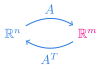
We can represent this relationship between matrix $A$, and its domain and codomain using a commutative diagram
Definition
A commutative diagram in linear algebra is a diagram of vector spaces and directed arrows that represent linear transformations so that any path along the arrows (composition of linear transformations) with the same starting vector space and ending vector space is equivalent.
Notice that in the commutative diagram we also depict the relationship between matrix $A^T$. The domain of $A^T$ is the codomain of $A$, and the codomain of $A^T$ is the domain of $A$.
Example 2 - RGB Color Space
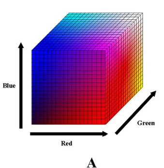
In the RGB color model, a 3-dimensional vector of integer values between 0 and 255 is modeled to be intensities of red, green, and blue. This is an additive color model so the absence of light, $\mathbf{0} = \langle 0,0,0 \rangle$ is black; the origin of the color space. The sum of all three colors at maximum intensity $\langle 255, 255, 255 \rangle$ is white; the far corner in the figure.
Hence of the infinite variety of possible hues, only $256^3 = 16,777,216$ colors can be represented in our computer model, and displayed by electronic devices such as televisions, computers and watches.
The value of 255 comes from the fact that in 8 bits (1 byte) the binary value $11111111 = 2^8-1 = 256-1 = 255$. The 256 values are used to store each color creating a color palette that contains $\left(2^8\right)^3 = 256^3 = 16,777,216$ colors. The image in figure 2 illustrates the linear transformation from $\mathbb{R}^3$ to the continuum of visible colors our eyes can detect. However we limit ourselves the subset of values from 0 to 255 in each of the coordinates in $\mathbb{R}^3$ to be the domain of our map. Similarly the image of our linear transformation contains only those frequencies of visible light corresponding in the RGB color palette. In the default color palette we have for vector $\langle R, G, B \rangle$,
$$ \begin{align*} \text{Intensity} &\qquad &I &= \dfrac{R + G + B}{3} \\ \\ \text{Saturation} &\qquad &S &= 1 - \min(R,G,B)/I \\ \\ \text{Hue} &\qquad &H &= \left\{\begin{array}{ccc} \cos^{-1}\left(\dfrac{(R-G) + (R-B)}{2\sqrt{(R-G)^2 + (R-B)(G-B)}}\right) & \ & \text{if } G > B \\ \\ 0 & \ & \text{if } G = B \\ \\ 360 - \cos^{-1}\left(\dfrac{(R-G) + (R-B)}{2\sqrt{(R-G)^2 + (R-B)(G-B)}}\right) & \ & \text{if } G < B \end{array} \right. \end{align*} $$
The RGB Color Space is not really a vector space. While color is additive and subtractive, there are several models for vector sums outside of the unit cube in $\mathbb{R}^3$. I admit I just wanted to include it somewhere. There are several models like RGB Color Space, that are not truly vector spaces. Vector spaces still help us understand them.

Definition
The Four Fundamental Subspaces of a Matrix
For any matrix $A\in\mathbb{R}^{m\times n}$ (or $\mathbb{C}^{m\times n}$), the four main subspaces are
$$ \begin{align*} 1.\ &\text{the row space } C(A^T)\subset\mathbb{R}^n \\ 2.\ &\text{the null space } N(A)\subset\mathbb{R}^n \\ 3.\ &\text{the column space } C(A)\subset\mathbb{R}^m \\ 4.\ &\text{the left null space } N(A^T)\subset\mathbb{R}^m \end{align*} $$
One can determine bases for the column space, row space and null space by reducing the matrix into reduced row echelon form and performing backward substitution. However this must be performed again on the transpose of the matrix to determine the left null space. There are other ways to determine the left null space if we know that it is a trivial subspace.
Video Lecture 1: The Four Fundamental Subspaces
 The Four Fundamental Subspaces
Example 3 - Find the Four Fundamental Subspaces
Determine bases for the 4 main subspaces of the following matrix,
$$ A = \begin{bmatrix}\ \ 2\ & -1\ &\ \ 0\ &\ \ 2\ &\ \ 2\ \\ \ \ 8\ & -3\ &\ \ 3\ &\ \ 7\ &\ 4\ \\ \ \ 10\ & -7\ & -4\ &\ \ 6\ &\ \ 6\ \end{bmatrix} $$
Solution:
$$ \begin{align*} A = \begin{bmatrix}\ \ 2\ & -1\ &\ \ 0\ &\ \ 2\ &\ \ 2\ \\ \ \ 8\ & -3\ &\ \ 3\ &\ \ 7\ &\ 4\ \\ \ \ 10\ & -7\ & -4\ &\ \ 6\ &\ \ 6\ \end{bmatrix} &\xrightarrow{\substack{R_2-4R_1 \\ R_3-5R_1}} \begin{bmatrix}\ \ 2\ & -1\ &\ \ 0\ &\ \ 2\ &\ \ 2\ \\ \ \ 0\ &\ \ 1\ &\ \ 3\ & -1\ & -4\ \\ \ \ 0\ & -2\ & -4\ & -4\ & -4\ \end{bmatrix}\xrightarrow{R_3+2R_2} \\ \\ \begin{bmatrix}\ \ 2\ & -1\ &\ \ 0\ &\ \ 2\ &\ \ 2\ \\ \ \ 0\ &\ \ 1\ &\ \ 3\ & -1\ & -4\ \\ \ \ 0\ &\ \ 0\ &\ \ 2\ & -6\ & -12\ \end{bmatrix} &\xrightarrow{R_3/2} \begin{bmatrix}\ \ 2\ & -1\ &\ \ 0\ &\ \ 2\ &\ \ 2\ \\ \ \ 0\ &\ \ 1\ &\ \ 3\ & -1\ & -4\ \\ \ \ 0\ &\ \ 0\ &\ \ 1\ & -3\ & -6\ \end{bmatrix} \xrightarrow{R_2-3R_3} \\ \\ \begin{bmatrix}\ \ 2\ & -1\ &\ \ 0\ &\ \ 2\ &\ \ 2\ \\ \ \ 0\ &\ \ 1\ &\ \ 0\ &\ \ 8\ &\ \ 14\ \\ \ \ 0\ &\ \ 0\ &\ \ 1\ & -3\ & -6\ \end{bmatrix} &\xrightarrow{R_1+R_2} \begin{bmatrix}\ \ 2\ &\ \ 0\ &\ \ 0\ &\ \ 10\ &\ \ 16\ \\ \ \ 0\ &\ \ 1\ &\ \ 0\ &\ \ 8\ &\ \ 14\ \\ \ \ 0\ &\ \ 0\ &\ \ 1\ & -3\ & -6\ \end{bmatrix} \xrightarrow{R_1/2} \\ \\ \begin{bmatrix}\ \ 1\ &\ \ 0\ &\ \ 0\ &\ \ 5\ &\ \ 8\ \\ \ \ 0\ &\ \ 1\ &\ \ 0\ &\ \ 8\ &\ \ 14\ \\ \ \ 0\ &\ \ 0\ &\ \ 1\ & -3\ & -6\ \end{bmatrix} \end{align*} $$
The pivot columns are the first, second and third columns. The pivot rows are the first, second and third rows. Performing backward substitution one obtains
$$ \begin{align*} x_4 &= s\in\mathbb{R} \\ x_5 &= t\in\mathbb{R} \\ x_3 &= 3s + 6t \\ x_2 &= -8s - 14t \\ x_1 &= -5s - 8t \\ \end{align*} $$
A basis for the column space has 3 vectors (pivot columns). A basis for the row space has 3 vectors (pivot rows). A basis for the null space has 2 vectors (free columns). Matrix $A^T$ has only 3 pivot columns (pivot rows) and no free columns so the left null space is trivial.
$$ \begin{align*} C(A) &= \text{Span}\left\{\,\begin{bmatrix}\ 2\ \\ \ 8\ \\ \ 10\ \end{bmatrix},\ \begin{bmatrix} -1\ \\ -3\ \\ -7\ \end{bmatrix},\ \begin{bmatrix}\ \ 0\ \\ \ \ 3\ \\ -4\ \end{bmatrix}\,\right\} \\ \\ C(A^T) &= \text{Span}\left\{\,\begin{bmatrix}\ 1\ \\ \ 0\ \\ \ 0\ \\ \ 5\ \\ \ 8\ \end{bmatrix},\ \begin{bmatrix}\ 0\ \\ \ 1\ \\ \ 0\ \\ \ 8\ \\ \ 14\ \end{bmatrix},\ \begin{bmatrix}\ \ 0\ \\ \ \ 0\ \\ \ \ 1\ \\ -3\ \\ -6\ \end{bmatrix}\,\right\} = \text{Span}\left\{\,\begin{bmatrix}\ \ 2\ \\ -1\ \\ \ \ 0\ \\ \ \ 2\ \\ \ \ 2\ \end{bmatrix},\ \begin{bmatrix}\ \ 8\ \\ -3\ \\ \ \ 3\ \\ \ \ 7\ \\ \ \ 4\ \end{bmatrix},\ \begin{bmatrix}\ \ 10\ \\ -7\ \\ -4\ \\ \ \ 6\ \\ \ \ 6\ \end{bmatrix}\,\right\} \\ \\ N(A) &= \text{Span}\left\{\,\begin{bmatrix} -5\ \\ -8\ \\ \ \ 3\ \\ \ \ 1\ \\ \ \ 0\ \end{bmatrix},\ \begin{bmatrix} -8\ \\ -14\ \\ \ \ 6\ \\ \ \ 0\ \\ \ \ 1\ \end{bmatrix}\,\right\} \end{align*} $$
All three rows of $A$ are pivot rows, therefore the left null space is trivial.
$$ N(A^T) = \left\{\,\mathbf{0}\,\right\} $$
Examining a pivot of an $m\times n$ matrix, the column containing the pivot is a pivot column, and the row containing the pivot is a pivot row. This means that the dimension of the column space always equals the dimension of the row space.
Theorem 1
The Row Space and the Column Space Have the Same Dimension
For any $m\times n$ matrix $A$, $\dim\left(C(A^T)\right) = \dim\left(C(A)\right)$.
Proof of Theorem 1
Let $A$ be an $m\times n$ matrix. Every pivot in a matrix identifies a single pivot row and a single pivot column. Using Theorem 4.5.8,
- The $\dim(C(A)) = $ the number of pivots in matrix $A$
- The $\dim(C(A^T)) = $ the number of pivots in matrix $A$
Therefore, the row space and the column space have the same dimension. $\blacksquare$
Definition
Rank
For any $m\times n$ matrix $A$, the dimension of the row space $C\left(A^T\right)$ is called the rank of matrix $A$.
It is curious that the rank is defined by the dimension of the row space. This is due to Theorem 4.5.7. Since we use elementary row operations to reduce a matrix, the row space is preserved. Notice that for any $m\times n$ matrix, the number of pivots $r$ must be less than or equal to the number of rows, $r \le m$. However it is also true that the number of pivots must also be less than or equal to the number of columns, $r \le n$. Thus if $r$ is the number of pivots in our reduced matrix,
$$ 0 \le r \le \min\left\{m, n \right\} $$
The only matrices with rank $0$ are the $m\times n$ zero matrices, $O$; they have no pivots.
Definition
Full Rank
If every column of matrix $A$ is a pivot column, we say that matrix $A$ has full rank.
In this case the rank of $m\times n$ matrix $A$ is equal to the number of columns, $n$.
Definition
Nullity
The dimension of the (right) null space of an $m\times n$ matrix $A$ is called the nullity of the matrix.
Since the rank $r = \dim\left(C(A)\right) = \dim\left(C(A^T)\right)$, then what does this mean for the right and left null space? Every column of a matrix must be either a free column or a pivot column, but not both. Therefore, $\mathrm{rank}(A) + \mathrm{nullity}(A) = n$, the number of columns. Similarly, $\mathrm{rank}(A^T) + \mathrm{nullity}(A^T) = m$.
Theorem 2
The Rank-Nullity Theorem
For any $m\times n$ matrix $A$ the rank of $A$ plus the nullity of $A$ equals $n$, the number of columns.
$$\text{rank}(A) + \text{nullity}(A) = n$$
You should convince yourself of the truth of this theorem using the theorems and definitions in this chapter.
If $A$ is an $m\times n$ matrix with rank $r$, then we can make several observations
- $\text{nullity}(A) = n - r$
- $\text{nullity}(A^T) = m-r$
- the number of pivot columns of $A = r$
- the number of pivot columns of $A^T = r$
- matrix $A$ has full rank if and only if $\text{nullity}(A)=0$
- a consistent linear system $A\mathbf{x}=\mathbf{b}$ has a unique solution if and only if $\text{nullity}(A)=0$
The concept of the vector sum of two subspaces of a vector space follows directly from the overlap (intersection) and accumulation (union) of sets.
One may form a new set from two sets that contains all of the elements in both sets. This is the intersection of sets. The intersection of two sets $E$ and $F$ is the set that contains all of the elements in both sets. This new set is denoted using the $\cap$ symbol
$$ E\cap F = \left\{\,x\,:\,x\in E\ \text{and}\ x\in F\,\right\} $$
Example 4
Suppose $E = \left\{ 1, 2, 3 \right\}$ and $F=\left\{3, 4, 5\right\}$, then
$$ E\cap F = \left\{\,3\,\right\} $$
Consider the following properties of subsets
$$ \begin{align*} E\cap \left\{\ \right\} &= E\cap\emptyset = \emptyset \\ \\ E\cap E &= E \\ \\ E\cap F &= F\cap E \end{align*} $$
If $E\subset F$, then $E\cap F = E$.
If $E\cap F = \emptyset$, then we say that the two sets are disjoint.
Subspaces of a vector space are subsets of the vector space. Remember that every subspace of a vector space must contain the zero vector, so subspaces are nonempty. Two subspaces always have a nonempty intersection since the zero vector is in both subspaces. Subspaces of a vector space are never disjoint. However their bases may not have any vectors in common.
Theorem 3
The intersection of two subspaces in a vector space is a subspace of the vector space.
If $U$ and $W$ are subspaces of vector space $V$, then a basis for $U\cap W$ can be extended to a basis for $U$ and extended to a basis for $W$. Hence
$$ \dim(U\cap W) \le \min\left\{\,\dim(U), \dim(W)\,\right\} $$
Proof of Theorem 3
Suppose that $U$ and $W$ are subspaces of vector space $V$. Then $U\cap W\neq\emptyset$ as the zero vector is in both $U$ and $W$.
Suppose further that $\mathbf{x},\ \mathbf{y}\in U\cap W$, and $s,\ t\in\mathbb{R}$. Then the linear combination $s\mathbf{x} + t\mathbf{y}\in U$ since $U$ is a subspace of $V$. Also $s\mathbf{x} + t\mathbf{y}\in W$ as $W$ is also a subspace of $V$. Since this vector is in both subspaces,
$$ s\mathbf{x} + t\mathbf{y}\in U\cap W $$
Since $U\cap W$ is closed under linear combinations, $U\cap W$ is a subspace of vector space $V$.
If $\mathfrak{B}$ is a basis for $U\cap W$, then $\mathfrak{B}$ can be extended to a basis for $U$ since $U\cap W$ is a subspace of $U$. Thus $\dim(U\cap W)\le\dim(U)$. Likewise $\mathfrak{B}$ can be extended to a basis for $W$ since $U\cap W$ is a subspace of $W$. Thus $\dim(U\cap W)\le\dim(W)$. Hence
$$ \dim(U\cap W)\le\min\left\{\,\dim(U),\ \dim(W)\,\right\}\ \blacksquare $$
One may also accumulate two subsets together into a larger set of the elements of either set. This is the
union. This new set is denoted using the $\cup$ symbol
$$E\cup F = \left\{\,x\,:\,x\in E,\ \text{or}\ x\in F\,\right\}$$
Example 5
Suppose $E = \left\{ 1, 2, 3 \right\}$ and $F=\left\{3, 4, 5\right\}$, then
$$ E\cup F = \left\{ 1, 2, 3, 4, 5 \right\} $$
Notice that 3 does not appear twice in $E\cup F$. Consider the following properties of subsets
$$ \begin{align*} E\cup \left\{\ \right\} &= E\cup\emptyset = E \\ \\ E\cup E &= E \\ \\ E\cup F &= F \cup E \\ \\ \text{If } E\subset F,&\text{ then } E\cup F = F. \end{align*} $$
If $U$ and $W$ are subspaces of vector space $V$, then we can form the union of these two sets, $U\cup W$, however the union is usually not a subspace.
Example 6
Suppose that $U = \text{Span}\left\{\ihat\right\}$ and $W = \text{Span}\left\{\jhat\right\}$ in vector space $\mathbb{R}^2$.
$$ \begin{align*} U\cup W &= \left\{\,c\ihat\,:\,c\in\mathbb{R}\,\right\}\cup\left\{\,d\jhat\,:\,d\in\mathbb{R}\,\right\} \\ \\ &= \left\{\,c\ihat,\ d\jhat\,:\,c,d\in\mathbb{R}\,\right\} \end{align*} $$
$U\cup W$ is the set of all scalar multiples of $\ihat$, and all scalar multiples of $\jhat$; is an infinitely large plus sign. Set $U\cup W$ is not closed under vector addition. $U\cup W$ does not contain $\ihat + \jhat$.
Definition
Vector Sum
The vector sum of two subspaces $U$ and $W$ of a vector space $V$ is the span of both vector spaces.
$$ U + W := \text{Span}\left\{ U\cup W \right\} $$
A vector sum yields a new subspace with all of the vectors in both subspaces, and all of their linear combinations. Now $U$ has a basis $\left\{\,\mathbf{u}_1,\ \dots,\ \mathbf{u}_r\,\right\}$, and $W$ has a basis $\left\{\,\mathbf{w}_1,\ \dots,\ \mathbf{w}_s\,\right\}$, and all of the vectors in either subspace is a linear combination of the basis vectors. If one notes that a linear combination of linear combinations is a linear combination we have the following theorem.
Theorem 4
The Union of Bases for the Vector Sum
If $U$ and $W$ are subspaces of vector space $V$, and the subspaces have bases
$$ \begin{align*} U &= \text{Span}\left\{\,\mathbf{u}_1,\ \dots,\ \mathbf{u}_r\,\right\} \\ W &= \text{Span}\left\{\,\mathbf{w}_1,\ \dots,\ \mathbf{w}_s\,\right\} \\ \end{align*} $$
then
$$ U + W = \text{Span}\left\{\,\mathbf{u}_1,\ \dots,\ \mathbf{u}_r,\mathbf{w}_1,\ \dots,\ \mathbf{w}_s\,\right\} $$
Since subspaces $U$ and $W$ may share basis vectors, or a basis vector for one subspace may be a vector in the other subspace,
$$ \dim(U + W) \le \dim(U) + \dim(W) $$
If the intersection of two subspaces is the trivial subspace $U\cap W = \left\{\mathbf{0}\right\}$, then clearly any bases of $U$ and $W$ will be disjoint.
Definition
Direct Sum
If $U$ and $W$ are subspaces of vector space $V$, and $U\cap W=\left\{\mathbf{0}\right\}$, then the vector sum of $U$ and $W$ is called a direct sum and denoted
$$ U\oplus W $$
A basis for $U\oplus W$ is the union of any two bases for $U$ and $W$, and
$$ \dim(U\oplus W) = \dim(U) + \dim(W) $$
The vector sum in example 6 is a direct sum because the horizontal axis $U = \textrm{Span}\left\{\ihat\right\}$, and the vertical axis $W = \textrm{Span}\left\{\jhat\right\}$ have only the origin in common.
Proof of Theorem 5
Let $A$ be an $m\times n$ matrix. If $\mathbf{x}\in\mathbb{R}^n$ is in both the null space $N(A)$ and the row space $C\left(A^T\right)$, then $A\mathbf{x} = \mathbf{0}$ and $\mathbf{x} = A^T\mathbf{y}$ for some $\mathbf{y}\in\mathbb{R}^m$. This gives us
$$ x_1^2 + x_2^2 + \cdots + x_n^2 = \mathbf{x}\cdot\mathbf{x} = \mathbf{x}^T\mathbf{x} = \left(\mathbf{y}^TA\right)\mathbf{x} = \mathbf{y}^T\left(A\mathbf{x}\right) = \mathbf{y}^T\mathbf{0} = 0. $$
A sum of nonnegative scalars is zero only when they are all zero, so $\mathbf{x}=\mathbf{0}$. Thus the row space and the null space have only the zero vector in common. $\blacksquare$
Replacing matrix $A$ with $A^T$ one obtains
$$ C(A)\cap N\left(A^T\right) = \left\{\mathbf{0}\right\} $$
Now the row space of $m\times n$ matrix $A$ has dimension $r =$ the rank$(A)$, the null space of matrix $A$ has dimension $n-r=$ the nullity$(A)$, and they have only the zero vector in common. Hence the vector sum of the row space $C(A^T)$ and the null space $N(A)$ has dimension $n$.
Theorem 6
If $A$ is an $m\times n$ matrix, then
$$ \begin{align*} C(A)\oplus N(A^T) &= \mathbb{R}^m \\ \\ C(A^T)\oplus N(A) &= \mathbb{R}^n \end{align*} $$
The rank-nullity theorem and Theorem 6 have other interesting implications for a linear system of equations.
Theorem 7
A linear system of equations $A\mathbf{x} = \mathbf{b}$ has at most one solution if and only if $N(A)=\left\{\mathbf{0}\right\}$. This means $$\mathrm{rank}(A) = n - \mathrm{nullity}(A) = n - 0 = n$$
A linear system of equations $A\mathbf{x} = \mathbf{b}$ has at least one solution if and only if $\mathbf{b}\in C(A)$.
A linear system of equations $A\mathbf{x} = \mathbf{b}$ has at most one solution if and only if $A$ has full rank.
If $n\times n$ linear system of equations $A\mathbf{x} = \mathbf{b}$ is consistent for every $\mathbf{b}\in\mathbb{R}^n$, then $N\left(A^T\right) = \left\{\mathbf{0}\right\}$ and $A$ must be a nonsingular matrix.
An $n\times n$ matrix $A$ is nonsingular if and only if the column vectors of $A$ form a basis for $\mathbb{R}^n$.
There are many similar conclusions one can make from the theorems of chapter 4. A student must become familiar enough with the important definitions and theorems to be able to understand when statements about linear systems are true and false. This is especially true for modern students. The linear systems of equations of interest are very large with possibly billions of unknowns and billions of equations. Only familiarity with the properties and theorems will help one understand these linear models.
Exercise 1
Let
$$
A = \begin{bmatrix}\ \ 1 &\ \ 2 &\ \ 8 &\ \ 0 &\ \ 4 \\
-2 &\ \ 2 &\ \ 2 & -4 &\ \ 2 \\
\ \ 2 & -3 & -5 &\ \ 2 & -1 \\
\ \ 1 & -2 & -4 & -1 &\ \ 1 \end{bmatrix}.
$$
Determine the four main subspaces of matrix $A$.
View Solution
We need to reduce matrix $A$ to upper triangular form. $$ \begin{align*} \begin{bmatrix}\ \ {\color{crimson} 1} &\ \ 2 &\ \ 8 &\ \ 0 &\ \ 4 \\ -2 &\ \ 2 &\ \ 2 & -4 &\ \ 2 \\ \ \ 2 & -3 & -5 &\ \ 2 & -1 \\ \ \ 1 & -2 & -4 & -1 &\ \ 1 \end{bmatrix} &\xrightarrow{\substack{R_2+2R_1 \\ R_3-2R_1 \\ R_4-R_1}} \begin{bmatrix}\ \ {\color{crimson} 1} &\ \ 2 &\ \ 8 &\ \ 0 &\ \ 4 \\ \ \ 0 &\ \ {\color{crimson} 6} &\ 18 & -4 &\ 10 \\ \ \ 0 & -7 & -21 &\ \ 2 & -9 \\ \ \ 0 & -4 & -12 & -1 & -3 \end{bmatrix} \xrightarrow{R_2+R_3} \begin{bmatrix}\ \ {\color{crimson} 1} &\ \ 2 &\ \ 8 &\ \ 0 &\ \ 4 \\ \ \ 0 & {\color{crimson} -1} & -3 & -2 &\ \ 1 \\ \ \ 0 & -7 & -21 &\ \ 2 & -9 \\ \ \ 0 & -4 & -12 & -1 & -3 \end{bmatrix} \xrightarrow{\substack{R_3-7R_2 \\ R_4-4R_2}} \\ \\ \begin{bmatrix}\ \ {\color{crimson} 1} &\ \ 2 &\ \ 8 &\ \ 0 &\ \ 4 \\ \ \ 0 & {\color{crimson} -1} & -3 & -2 &\ \ 1 \\ \ \ 0 &\ \ 0 &\ \ 0 & {\color{crimson} 16} & -16 \\ \ \ 0 &\ \ 0 &\ \ 0 & 7 & -7 \end{bmatrix} &\xrightarrow{\substack{-R_2 \\ R_3/16}} \begin{bmatrix}\ \ {\color{crimson} 1} &\ \ 2 &\ \ 8 &\ \ 0 &\ \ 4 \\ \ \ 0 &\ \ {\color{crimson} 1} &\ \ 3 &\ \ 2 & -1 \\ \ \ 0 &\ \ 0 &\ \ 0 &\ \ {\color{crimson} 1} & -1 \\ \ \ 0 &\ \ 0 &\ \ 0 &\ \ 7 & -7 \end{bmatrix} \xrightarrow{R_4-7R_3} \begin{bmatrix}\ \ {\color{crimson} 1} &\ \ 2 &\ \ 8 &\ \ 0 &\ \ 4 \\ \ \ 0 &\ \ {\color{crimson} 1} &\ \ 3 &\ \ 2 & -1 \\ \ \ 0 &\ \ 0 &\ \ 0 &\ \ {\color{crimson} 1} & -1 \\ \ \ 0 &\ \ 0 &\ \ 0 &\ \ 0 &\ \ 0\ \end{bmatrix} = U \\ \end{align*} $$
Matrix $U$ has $3$ pivot columns, so matrix $A$ has three pivot columns. The rank$(A) = 3$.
The column space of matrix $A$ consists of the span of the $3$ pivot columns of matrix $A$. We must use the original three pivot columns of matrix $A$ because we performed row operations and row operations destroy the column space.
$$ C(A) = \text{Span} \left\{\,\mathbf{a}_1, \mathbf{a}_2, \mathbf{a}_4\,\right\} = \text{Span}\left\{\,\begin{bmatrix}\ \ 1 \\ -2 \\ \ \ 2 \\ \ \ 1 \end{bmatrix},\ \begin{bmatrix}\ \ 2 \\ \ \ 2 \\ -3 \\ -2 \end{bmatrix},\ \begin{bmatrix}\ \ 0 \\ -4 \\ \ \ 2 \\ -1 \end{bmatrix}\,\right\} $$
The row space of matrix $A$ consists of the span of the $3$ pivot columns of $A^T$. Since row operations are linear combinations of the rows of matrix $A$, row operations preserve the row space. We may use the rows of $U$ or the rows of row equivalent matrix $A$.
$$ \begin{align*} C\left(A^T\right) &= \text{Span} \left\{\,\begin{bmatrix} 1 \\ 2 \\ 8 \\ 0 \\ 4 \end{bmatrix},\ \begin{bmatrix} -2 \\ \ \ 2 \\ \ \ 2 \\ -4 \\ \ \ 2 \end{bmatrix},\ \begin{bmatrix}\ \ 2 \\ -3 \\ -5 \\ \ \ 2 \\ -1 \end{bmatrix}\,\right\} \\ \\ &= \text{Span} \left\{\,\begin{bmatrix} 1 \\ 2 \\ 8 \\ 0 \\ 4 \end{bmatrix},\ \begin{bmatrix}\ \ 0 \\ \ \ 1 \\ \ \ 3 \\ \ \ 2 \\ -1 \end{bmatrix},\ \begin{bmatrix}\ \ 0 \\ \ \ 0 \\ \ \ 0 \\ \ \ 1 \\ -1 \end{bmatrix}\,\right\} \\ \end{align*} $$
We must complete backward substitution for $A\mathbf{x} = \mathbf{0}$ to obtain the null space. Let us start by reducing $U$ to reduced row echelon form $R$.
$$ \begin{align*} \begin{bmatrix}\ \ 1 &\ \ 2 &\ \ 8 &\ \ 0 &\ \ 4 \\ \ \ 0 &\ \ 1 &\ \ 3 &\ \ 2 & -1 \\ \ \ 0 &\ \ 0 &\ \ 0 &\ \ 1 & -1 \\ \ \ 0 &\ \ 0 &\ \ 0 &\ \ 0 &\ \ 0 \end{bmatrix} \xrightarrow{R_2-2R_3} \begin{bmatrix}\ \ 1 &\ \ 2 &\ \ 8 &\ \ 0 &\ \ 4 \\ \ \ 0 &\ \ 1 &\ \ 3 &\ \ 0 &\ \ 1 \\ \ \ 0 &\ \ 0 &\ \ 0 &\ \ 1 & -1 \\ \ \ 0 &\ \ 0 &\ \ 0 &\ \ 0 &\ \ 0 \end{bmatrix} \xrightarrow{R_1-2R_2} \begin{bmatrix}\ \ 1 &\ \ 0 &\ \ 2 &\ \ 0 &\ \ 2 \\ \ \ 0 &\ \ 1 &\ \ 3 &\ \ 0 &\ \ 1 \\ \ \ 0 &\ \ 0 &\ \ 0 &\ \ 1 & -1 \\ \ \ 0 &\ \ 0 &\ \ 0 &\ \ 0 &\ \ 0 \end{bmatrix} \end{align*} $$
Now for backward substitution
$$ \begin{align*} x_3 &= \alpha\in\mathbb{R} \\ x_5 &= \beta\in\mathbb{R} \\ \\ x_4 - \beta &= 0 \\ x_4 &= \beta \\ \\ x_2 + 3\alpha + \beta &= 0 \\ x_2 &= -3\alpha - \beta \\ \\ x_1 + 2\alpha + 2\beta &= 0 \\ x_1 &= -2\alpha -2\beta \\ \\ N(A) &= \left\{\,\begin{bmatrix} -2\alpha - 2\beta \\ -3\alpha - \beta \\ \alpha \\ \beta \\ \beta \end{bmatrix}\,:\,\alpha,\beta\in\mathbb{R}\,\right\} \\ \\ &= \left\{\,\alpha\begin{bmatrix} -2 \\ -3 \\ 1 \\ 0 \\ 0 \end{bmatrix} + \beta\begin{bmatrix} -2 \\ -1 \\ 0 \\ 1 \\ 1 \end{bmatrix}\,:\,\alpha\beta\in\mathbb{R}\,\right\} \\ \\ &= \text{Span}\left\{\,\begin{bmatrix} -2 \\ -3 \\ 1 \\ 0 \\ 0 \end{bmatrix},\ \begin{bmatrix} -2 \\ -1 \\ 0 \\ 1 \\ 1 \end{bmatrix}\,\right\} \end{align*} $$
To determine the null space of $A^T$ we must reduce $A^T$ enough to use backward substitution.
$$ \begin{align*} \begin{bmatrix}\ \ 1 & -2 &\ \ 2 &\ \ 1 \\ \ \ 2 &\ \ 2 & -3 & -2 \\ \ \ 8 &\ \ 2 & -5 & -4 \\ \ \ 0 & -4 &\ \ 2 & -1 \\ \ \ 4 &\ \ 2 & -1 &\ \ 1 \end{bmatrix} &\xrightarrow{\substack{R_2-2R_1 \\ R_3-8R_1 \\ R_5-4R_1}} \begin{bmatrix}\ \ 1 & -2 &\ \ 2 &\ \ 1 \\ \ \ 0 &\ \ 6 & -7 & -4 \\ \ \ 0 &\ 18 & -21 & -12 \\ \ \ 0 & -4 &\ \ 2 & -1 \\ \ \ 0 &\ 10 & -9 & -3 \end{bmatrix} \xrightarrow{R_2+R_4} \begin{bmatrix}\ \ 1 & -2 &\ \ 2 &\ \ 1 \\ \ \ 0 &\ \ 2 & -5 & -5 \\ \ \ 0 &\ 18 & -21 & -12 \\ \ \ 0 & -4 &\ \ 2 & -1 \\ \ \ 0 &\ 10 & -9 & -3 \end{bmatrix} \xrightarrow{\substack{R_3-9R_2 \\ R_4+2R_2 \\ R_5-5R_2}} \\ \\ \begin{bmatrix}\ \ 1 & -2 &\ \ 2 &\ \ 1 \\ \ \ 0 &\ \ 2 & -5 & -5 \\ \ \ 0 &\ \ 0 & 24 & 33 \\ \ \ 0 &\ \ 0 & -8 & -11 \\ \ \ 0 &\ \ 0 & 16 & 22 \end{bmatrix} &\xrightarrow{R_3-R_5} \begin{bmatrix}\ \ 1 & -2 &\ \ 2 &\ \ 1 \\ \ \ 0 &\ \ 2 & -5 & -5 \\ \ \ 0 &\ \ 0 &\ \ 8 & 11 \\ \ \ 0 &\ \ 0 & -8 & -11 \\ \ \ 0 &\ \ 0 & 16 & 22 \end{bmatrix} \xrightarrow{\substack{R_4+R_3 \\ R_5-2R_3}} \begin{bmatrix}\ \ 1 & -2 &\ \ 2 &\ \ 1 \\ \ \ 0 &\ \ 2 & -5 & -5 \\ \ \ 0 &\ \ 0 &\ \ 8 & 11 \\ \ \ 0 &\ \ 0 &\ \ 0 &\ \ 0 \\ \ \ 0 &\ \ 0 &\ \ 0 &\ \ 0 \end{bmatrix} \xrightarrow{R_1+R_2} \\ \\ \begin{bmatrix}\ \ 1 &\ \ 0 & -3 & -4 \\ \ \ 0 &\ \ 2 & -5 & -5 \\ \ \ 0 &\ \ 0 &\ \ 8 & 11 \\ \ \ 0 &\ \ 0 &\ \ 0 &\ \ 0 \\ \ \ 0 &\ \ 0 &\ \ 0 &\ \ 0 \end{bmatrix} &\xrightarrow{\substack{8R_1 \\ 8R_2}} \begin{bmatrix}\ \ 8 &\ \ 0 & -24 & -32 \\ \ \ 0 & 16 & -40 & -40 \\ \ \ 0 &\ \ 0 &\ \ 8 & 11 \\ \ \ 0 &\ \ 0 &\ \ 0 &\ \ 0 \\ \ \ 0 &\ \ 0 &\ \ 0 &\ \ 0 \end{bmatrix} \xrightarrow{\substack{R_1+3R_3 \\ R_2+5R_3}} \begin{bmatrix}\ \ 8 &\ \ 0 &\ \ 0 &\ \ 1 \\ \ \ 0 & 16 &\ \ 0 & 15 \\ \ \ 0 &\ \ 0 &\ \ 8 & 11 \\ \ \ 0 &\ \ 0 &\ \ 0 &\ \ 0 \\ \ \ 0 &\ \ 0 &\ \ 0 &\ \ 0 \end{bmatrix} \\ \\ x_4 &= 16\alpha\in\mathbb{R} \\ \\ 8x_3 + 11\cdot16\alpha &= 0 \\ x_3 &= -22\alpha \\ \\ 16x_2 + 15\cdot16\alpha &= 0 \\ x_2 &= -15\alpha \\ \\ 8x_1 + 16\alpha &= 0 \\ x_1 &= -2\alpha \\ N\left(A^T\right) &= \left\{\,\begin{bmatrix} -2\alpha \\ -15\alpha \\ -22\alpha \\ 16\alpha \end{bmatrix}\,:\,\alpha\in\mathbb{R}\,\right\} \\ \\ &= \text{Span}\left\{\,\begin{bmatrix} -2 \\ -15 \\ -22 \\ 16 \end{bmatrix}\,\right\} \end{align*} $$
Exercise 2
Determine the rank factorization of the matrix $A$ in Exercise 1
View Solution
We have$$ A = \begin{bmatrix}\ \ 1 &\ \ 2 &\ \ 8 &\ \ 0 &\ \ 4 \\ -2 &\ \ 2 &\ \ 2 & -4 &\ \ 2 \\ \ \ 2 & -3 & -5 &\ \ 2 & -1 \\ \ \ 1 & -2 & -4 & -1 &\ \ 1 \end{bmatrix}\qquad\qquad \text{rref}(A) = \begin{bmatrix}\ \ 1 &\ \ 0 &\ \ 2 &\ \ 0 &\ \ 2 \\ \ \ 0 &\ \ 1 &\ \ 3 &\ \ 0 &\ \ 1 \\ \ \ 0 &\ \ 0 &\ \ 0 &\ \ 1 & -1 \\ \ \ 0 &\ \ 0 &\ \ 0 &\ \ 0 &\ \ 0 \end{bmatrix} $$
So
$$ C = \begin{bmatrix} \mathbf{a}_1 & \mathbf{a}_2 & \mathbf{a}_4 \end{bmatrix} = \begin{bmatrix}\ \ 1 &\ \ 2 &\ \ 0 \\ -2 &\ \ 2 & -4 \\ \ \ 2 & -3 &\ \ 2 \\ \ \ 1 & -2 & -1 \end{bmatrix} $$
and matrix $R$ is the reduced row echelon form of $A$ with the rows of zeros removed...
$$ R = \begin{bmatrix}\ \ 1 &\ \ 0 &\ \ 2 &\ \ 0 &\ \ 2 \\ \ \ 0 &\ \ 1 &\ \ 3 &\ \ 0 &\ \ 1 \\ \ \ 0 &\ \ 0 &\ \ 0 &\ \ 1 & -1 \end{bmatrix} $$
Exercise 3
Using matrix $A$ from exercise 1, if $\mathbf{b}\in C(A)$, then how many solutions has the linear system $A\mathbf{x} = \mathbf{b}$?
View Solution
The nullity$(A) = 2 \gt 0$, so the null space is nontrivial. As $\mathbf{b}\in C(A)$, the system is consistent. Since the null space is nontrivial, there are infinitely many solutions.Exercise 4
Given two subspaces $U = \left\{ \langle x, x, 0 \rangle\,:\,x\in\mathbb{R}\,\right\}$, and $V = \left\{ \langle x, 0, y \rangle \,:\,x,y\in\mathbb{R} \,\right\}$, find $U + V$.
View Solution
The variables used in a definition of any aggregate mathematical object is a dummy variable. Any letter not already in use will do. The dummy variable has no existence outside of the definition of the set. So the variable $x$ in the definitions of $U$ and $V$ are actually different dummy variables. They cannot be used outside of each definition of the subspace. They cannot be combined or used across definitions to create unions, intersections, or vector sums.
The easiest way to describe any subspace is as the span of basis vectors in the subspace, or as a linear combination.
$$ \begin{align*} U &= \left\{\, \left. \begin{bmatrix}\ x\ \\ \ x\ \\ \ 0\ \end{bmatrix}\,\right|\, x\in\mathbb{R} \,\right\} = \left\{\, \left. x\begin{bmatrix}\ 1\ \\ \ 1\ \\ \ 0\ \end{bmatrix}\,\right|\, x\in\mathbb{R} \,\right\} = \textrm{Span}\left\{ \begin{bmatrix}\ 1\ \\ \ 1\ \\ \ 0\ \end{bmatrix} \,\right\} \\ \\ V &= \left\{\, \left. \begin{bmatrix}\ x\ \\ \ 0\ \\ \ y\ \end{bmatrix}\, \right|\, x,y\in\mathbb{R} \,\right\} = \left\{\, \left. \begin{bmatrix}\ x\ \\ \ 0\ \\ \ 0\ \end{bmatrix} + \begin{bmatrix}\ 0\ \\ \ 0\ \\ \ y\ \end{bmatrix}\, \right|\, x,y\in\mathbb{R} \,\right\} = \left\{\, \left. x\begin{bmatrix}\ 1\ \\ \ 0\ \\ \ 0\ \end{bmatrix} + y\begin{bmatrix}\ 0\ \\ \ 0\ \\ \ 1\ \end{bmatrix}\, \right|\, x,y\in\mathbb{R} \,\right\} = \textrm{Span}\left\{\, \ihat,\ \khat \,\right\} \\ \\ U + V &= \textrm{Span}\left\{\,\begin{bmatrix}\ 1\ \\ \ 1\ \\ \ 0\ \end{bmatrix},\ \ihat,\ \khat \,\right\} \\ \end{align*} $$
Now is this set a basis for $U+V$? It is a spanning set, but are the vectors linearly independent? What is the best way we have to determine which vectors are dependent? Create a matrix with these vectors as columns and reduce it until we know which are pivot columns and which are free columns (linear dependent).
$$ \begin{align*} \begin{bmatrix}\ 1\ &\ 1\ &\ 0\ \\ \ 1\ &\ 0\ &\ 0\ \\ \ 0\ &\ 0\ &\ 1\ \end{bmatrix}\begin{array}{l} R_2 \\ R_1 \\ \\ \end{array} &\rightarrow \begin{bmatrix}\ 1\ &\ 0\ &\ 0\ \\ \ 1\ &\ 1\ &\ 0\ \\ \ 0\ &\ 0\ &\ 1\ \end{bmatrix}\begin{array}{l} \\ R_2-R_1 \\ \\ \end{array} \rightarrow \begin{bmatrix}\ 1\ &\ 0\ &\ 0\ \\ \ 0\ &\ 1\ &\ 0\ \\ \ 0\ &\ 0\ &\ 1\ \end{bmatrix} \end{align*} $$
All three columns are pivot columns so this set of three vectors that spans $\mathbb{R}^3$ is a basis for $\mathbb{R}^3$. Hence $U+V=\mathbb{R}^3$. Another good way to check is to create the picture of the line $U$ and the plane $V$,
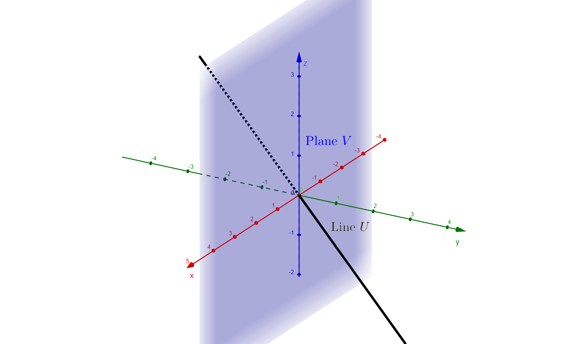
Since the intersection of subspaces $U$ and $V$ is the trivial subspace $\left\{\mathbf{0}\right\}$, this vector sum is a direct sum.
$$ U \oplus V = \mathbb{R}^3 $$
