

Exercise 1
Express each vector in standard coordinates $(x,y)\in\mathbb{R}^2$ relative to the basis
$$ \Theta = \left\{\begin{bmatrix} \cos(\theta) \\ \sin(\theta) \end{bmatrix},\ \begin{bmatrix} -\sin(\theta) \\ \ \ \cos(\theta) \end{bmatrix} \right\} $$
for any angle $\theta$ in radians.
Follow Along
We need to find the transition matrix from the standard coordinate system to the non-standard coordinate system $\Theta$. We start with the simpler to construct transition matrix from the new coordinate system to this standard coordinate system$$ T = \begin{bmatrix} \cos(\theta) & -\sin(\theta) \\ \sin(\theta) &\ \ \cos(\theta) \end{bmatrix} $$
$T^{-1}$ is the transition matrix from the standard coordinate system to the new coordinate system.
$$ \begin{align*} T^{-1} &= \frac{1}{\left|T\right|}\text{adj}(T) \\ \\ &= \frac{1}{\cos^2(\theta) + \sin^2(\theta)}\ \begin{bmatrix} \cos(\theta) & -\sin(\theta) \\ \sin(\theta) &\ \ \cos(\theta) \end{bmatrix}^T \\ \\ &= \begin{bmatrix}\ \ \cos(\theta) & \sin(\theta) \\ -\sin(\theta) & \cos(\theta) \end{bmatrix} \end{align*} $$
Now we can compute the coordinates of the vector $(x,y)$ in standard coordinates relative to the new coordinate system $\Theta$.
$$ T^{-1}\begin{bmatrix} x \\ y \end{bmatrix} = \begin{bmatrix}\ \ x\cos(\theta) + y\sin(\theta) \\ -x\sin(\theta) + y\cos(\theta) \end{bmatrix}_{\Theta} $$
Everything in this course works over any field of scalars, not only the real numbers. Digital hardware uses the field $\mathbb{F}_2 = \mathrm{GF}(2)$, whose only scalars are $0$ and $1$: addition is exclusive-or ($1 + 1 = 0$) and multiplication is and. Vectors are bit-strings, and linearly independent, span, rank, and null space mean exactly what they have always meant.
Definition - Binary Linear Code
A binary linear code is a subspace $C \subseteq \mathbb{F}_2^{\,n}$. It is described by either
- a generator matrix $G$ whose rows form a basis for $C$, so a message $\mathbf{m}$ is encoded as the codeword $\mathbf{c} = \mathbf{m}G$ and the code is the row space of $G$, or
- a parity-check matrix $H$ for which $C$ is the null space, so $\mathbf{c}$ is a codeword exactly when $H\mathbf{c} = \mathbf{0}$.
These are one subspace seen two ways, and the rank-nullity theorem links them: $\dim C = n - \mathrm{rank}(H)$. More data per block means a larger subspace, which means fewer parity checks.
Example 1 - The Hamming (7,4) Code
Four data bits are transmitted as seven using
$$ G = \begin{bmatrix} 1&0&0&0&1&1&0 \\ 0&1&0&0&0&1&1 \\ 0&0&1&0&1&1&1 \\ 0&0&0&1&1&0&1 \end{bmatrix}, \qquad H = \begin{bmatrix} 1&0&1&1&1&0&0 \\ 1&1&1&0&0&1&0 \\ 0&1&1&1&0&0&1 \end{bmatrix}. $$
Matrix $G$ has rank $4$, so $C$ is a $4$-dimensional subspace of $\mathbb{F}_2^{\,7}$ — that is $2^4 = 16$ codewords out of $128$ possible strings. Equivalently $\mathrm{rank}(H) = 3$, and $\dim C = 7 - 3 = 4$. One checks that $GH^T = 0$, so every row of $G$ lies in the null space of $H$.
Encode the message $\mathbf{m} = \begin{bmatrix} 1&0&1&1 \end{bmatrix}$:
$$ \mathbf{c} = \mathbf{m}G = \begin{bmatrix} 1&0&1&1&1&0&0 \end{bmatrix}, \qquad H\mathbf{c} = \mathbf{0} $$
confirms it is a codeword.
Now corrupt one bit in transmission — say bit $5$ flips, so the receiver gets $\mathbf{r} = \begin{bmatrix} 1&0&1&1&0&0&0 \end{bmatrix}$. The syndrome is
$$ \mathbf{s} = H\mathbf{r} = \begin{bmatrix} 1 \\ 0 \\ 0 \end{bmatrix}. $$
Here is the whole idea. If $\mathbf{r} = \mathbf{c} + \mathbf{e}$ where $\mathbf{e}$ is a single-bit error in position $j$, then
$$ H\mathbf{r} = H\mathbf{c} + H\mathbf{e} = H\mathbf{e} = \left(\text{column } j \text{ of } H\right). $$
The syndrome is literally a column of $H$, and it names the broken bit: the vector $\begin{bmatrix} 1&0&0 \end{bmatrix}^T$ is column $5$ of $H$, so bit $5$ is wrong. Flip it back and the message is recovered.
A code that pinpoints any single error needs its $H$-columns distinct and nonzero, which forces $2^3 - 1 \ge 7$ — the reason the $7$ and the $3$ in Hamming $(7,4)$ are what they are. This is why a QR code still scans with a coffee stain on it, and why 5G, solid-state drives, and the Voyager probes keep working over noisy channels. Industrial codes (Reed–Solomon in QR codes) use the same subspace and null-space structure over a larger field so they can repair whole bursts of errors.
Exercise 2
Using the matrix $H$ above, a receiver gets $\mathbf{r} = \begin{bmatrix} 1&1&1&0&1&0&1 \end{bmatrix}$. Compute the syndrome $H\mathbf{r}$, identify the single bit in error, correct it, and recover the four-bit message.
View Solution
The syndrome is the matrix-vector product $H\mathbf{r}$ computed over $\mathbb{F}_2$.$$ \mathbf{s} = H\mathbf{r} = \begin{bmatrix} 1&0&1&1&1&0&0 \\ 1&1&1&0&0&1&0 \\ 0&1&1&1&0&0&1 \end{bmatrix}\begin{bmatrix} 1\\1\\1\\0\\1\\0\\1 \end{bmatrix} = \begin{bmatrix} 1\\1\\1 \end{bmatrix} $$
The syndrome $\begin{bmatrix} 1&1&1 \end{bmatrix}^T$ is column $3$ of $H$, so bit $3$ is in error. Flipping bit $3$ of $\mathbf{r}$ produces a codeword,
$$ \mathbf{c} = \begin{bmatrix} 1&1&0&0&1&0&1 \end{bmatrix}, \qquad H\mathbf{c} = \mathbf{0}. $$
Because $G$ is in the systematic form $\begin{bmatrix} I_4 & P \end{bmatrix}$, the message is the first four bits of the codeword,
$$ \mathbf{m} = \begin{bmatrix} 1&1&0&0 \end{bmatrix}. $$
Recall from change of basis that the transition matrix from a frame to the standard (world) frame has the frame's basis vectors as its columns, written in world coordinates. In three dimensions the workhorses are the axis rotations
$$ R_z(\theta) = \begin{bmatrix} \cos\theta & -\sin\theta & 0 \\ \sin\theta & \cos\theta & 0 \\ 0 & 0 & 1 \end{bmatrix}, \qquad R_x(\theta) = \begin{bmatrix} 1 & 0 & 0 \\ 0 & \cos\theta & -\sin\theta \\ 0 & \sin\theta & \cos\theta \end{bmatrix}, $$
each a transition matrix from a rotated frame back to world coordinates.
Example 2 - Composing Frames
Suppose an object's frame is the world frame rotated $90^\circ$ about the $z$-axis and then $90^\circ$ about the $x$-axis. The transition matrix from object coordinates to world coordinates is the product
$$ T = R_x(90^\circ)\,R_z(90^\circ) = \begin{bmatrix} 0 & -1 & 0 \\ 0 & 0 & -1 \\ 1 & 0 & 0 \end{bmatrix}. $$
Its columns are the object's three axes as seen from the world. A point at $\begin{bmatrix} 1&0&0 \end{bmatrix}^T$ in the object frame sits at $T\begin{bmatrix} 1&0&0 \end{bmatrix}^T = \begin{bmatrix} 0&0&1 \end{bmatrix}^T$ in the world. To carry a world point into object coordinates, multiply by $T^{-1}$, just as $T^{-1}$ carried standard coordinates into $\Theta$-coordinates in the rotation-of-axes example.
The modern payoff is composition. A game engine sends a model through model $\to$ world $\to$ camera $\to$ screen, each arrow a transition matrix and the whole pipeline their product. A robot arm stacks one transition matrix per joint, so the gripper's position in the world is the product of the joint matrices (forward kinematics). A self-driving car fuses a LIDAR return by pushing it through sensor $\to$ vehicle $\to$ world. It is all change of basis, multiplied together.
Two practical notes. A rotation carries points but not translation; to include a shift $\mathbf{t}$, graphics uses homogeneous coordinates, writing each point as $\begin{bmatrix} x&y&z&1 \end{bmatrix}^T$ and each frame as the $4 \times 4$ matrix $\begin{bmatrix} R & \mathbf{t} \\ \mathbf{0} & 1 \end{bmatrix}$, so that composing frames stays plain matrix multiplication. Also, these rotation matrices satisfy $T^{-1} = T^T$ — a preview of orthogonality from later in the course. For now you can invert $T$ by the usual method and treat the transpose as a shortcut to be justified then.
Exercise 3
A camera frame is the world rotated $-90^\circ$ about the $z$-axis. Write its transition matrix $T$ (world $\leftarrow$ camera), and find where the world point $\begin{bmatrix} 2&1&0 \end{bmatrix}^T$ lands in camera coordinates. Then compose with a second frame rotated $90^\circ$ about the $x$-axis and give the single matrix that carries the second frame's coordinates all the way to the world.
View Solution
The camera frame is the world rotated $-90^\circ$ about the $z$-axis, so the transition matrix to the world has the rotated axes as its columns,$$ T = R_z(-90^\circ) = \begin{bmatrix} \ \ 0 & 1 & 0 \\ -1 & 0 & 0 \\ \ \ 0 & 0 & 1 \end{bmatrix}. $$
To express the world point $\begin{bmatrix} 2&1&0 \end{bmatrix}^T$ in camera coordinates, multiply by $T^{-1} = T^T$,
$$ \begin{bmatrix} 2\\1\\0 \end{bmatrix}_{\text{cam}} = T^{-1}\begin{bmatrix} 2\\1\\0 \end{bmatrix} = \begin{bmatrix} \ \ 0 & -1 & 0 \\ \ \ 1 & \ \ 0 & 0 \\ \ \ 0 & \ \ 0 & 1 \end{bmatrix}\begin{bmatrix} 2\\1\\0 \end{bmatrix} = \begin{bmatrix} -1\\ \ \ 2\\ \ \ 0 \end{bmatrix}_{\text{cam}}. $$
A second frame rotated $90^\circ$ about the $x$-axis relative to the camera has transition matrix $R_x(90^\circ)$ into the camera frame. Composing second $\to$ camera with camera $\to$ world gives the single matrix from the second frame all the way to the world,
$$ T\,R_x(90^\circ) = \begin{bmatrix} \ \ 0 & 1 & 0 \\ -1 & 0 & 0 \\ \ \ 0 & 0 & 1 \end{bmatrix}\begin{bmatrix} 1 & 0 & \ \ 0 \\ 0 & 0 & -1 \\ 0 & 1 & \ \ 0 \end{bmatrix} = \begin{bmatrix} \ \ 0 & 0 & -1 \\ -1 & 0 & \ \ 0 \\ \ \ 0 & 1 & \ \ 0 \end{bmatrix}. $$
The JPEG standard is two changes of basis, each chosen so that the coordinate list of a natural image is mostly tiny numbers — which are then discarded.
Color, in a better basis. A pixel is a vector $\begin{bmatrix} R&G&B \end{bmatrix}^T$. The eye is far more sensitive to brightness than to color detail, but the RGB basis mixes the two together. JPEG first changes basis to separate luminance $Y$ from two chrominance channels $C_b$ and $C_r$:
$$ \begin{bmatrix} Y \\ C_b \\ C_r \end{bmatrix} = \begin{bmatrix} \ \ 0.299 & \ \ 0.587 & \ \ 0.114 \\ -0.169 & -0.331 & \ \ 0.500 \\ \ \ 0.500 & -0.419 & -0.081 \end{bmatrix} \begin{bmatrix} R \\ G \\ B \end{bmatrix} \quad (+\text{ offsets on } C_b,\ C_r). $$
Example 3 - Color in a Better Basis
Pure red $\begin{bmatrix} 255&0&0 \end{bmatrix}^T$ becomes about $\begin{bmatrix} 76&85&255 \end{bmatrix}^T$, white $\begin{bmatrix} 255&255&255 \end{bmatrix}^T$ becomes $\begin{bmatrix} 255&128&128 \end{bmatrix}^T$, and any gray $\begin{bmatrix} g&g&g \end{bmatrix}^T$ becomes $\begin{bmatrix} g&128&128 \end{bmatrix}^T$ — all of its information in $Y$, none in the color channels. The matrix is invertible, so the change of basis itself loses nothing; the compression comes next, when the $C_b$ and $C_r$ channels are stored at reduced resolution because the eye does not notice.
Shape, in a better basis. Within a channel the image is cut into $8 \times 8$ blocks — each a vector in $\mathbb{R}^{64}$ — and re-expressed in the discrete cosine transform (DCT) basis, whose basis vectors are sampled cosine waves of increasing frequency. Because natural image blocks are smooth, almost all of their DCT coordinates are near zero.
Example 4 - The Discrete Cosine Transform
The one-dimensional version shows the whole story. Take the orthonormal $8$-point DCT basis, whose transition matrix $C$ has the cosine vectors as its rows, and the smooth signal $\mathbf{f} = \begin{bmatrix} 50&52&55&60&62&61&58&54 \end{bmatrix}^T$. Its coordinates are
$$ C\mathbf{f} = \begin{bmatrix} 159.8 & -6.3 & -9.5 & 2.4 & 0.0 & 0.4 & -0.7 & -0.2 \end{bmatrix}^T. $$
The last four coordinates are negligible. Keep only the first four, discard the rest, and reconstruct:
$$ \begin{bmatrix} 50.0 & 51.8 & 55.4 & 59.6 & 62.2 & 61.3 & 57.6 & 54.2 \end{bmatrix}^T, $$
off by at most $0.45$ from the original — half the data, essentially the same signal. Compression is choosing a basis in which the coordinate list collapses to a few significant numbers, then dropping the rest. JPEG's quantization step is exactly this rounding of the small DCT coordinates to zero.
Here the DCT basis is orthonormal, so $C^{-1} = C^T$ — again the orthogonality result from later in the course. Until then, the coordinates can be obtained by solving the change-of-basis system with $C^{-1}$ directly; nothing in the compression idea needs more than that.
Exercise 4
(a) Using the color matrix above, find the $Y$, $C_b$, and $C_r$ values (before offsets) of the pixel $\begin{bmatrix} 100&150&200 \end{bmatrix}^T$, and confirm that a gray pixel $\begin{bmatrix} g&g&g \end{bmatrix}^T$ always gives $C_b = C_r = 0$ before offsets.
(b) A block's DCT coordinates are $\begin{bmatrix} 200 & 15 & -4 & 3 & 0.2 & -0.1 & 0 & 0.05 \end{bmatrix}^T$. If you keep only the coordinates larger than $1$ in absolute value, how many of the eight do you store, and what compression ratio is that for the block?
View Solution
(a) Multiply the pixel by the color matrix (before offsets),$$ \begin{bmatrix} Y\\C_b\\C_r \end{bmatrix} = \begin{bmatrix} \ \ 0.299 & \ \ 0.587 & \ \ 0.114 \\ -0.169 & -0.331 & \ \ 0.500 \\ \ \ 0.500 & -0.419 & -0.081 \end{bmatrix}\begin{bmatrix} 100\\150\\200 \end{bmatrix} = \begin{bmatrix} 140.75\\ \ \ 33.45\\ -29.05 \end{bmatrix}. $$
For a gray pixel $\begin{bmatrix} g&g&g \end{bmatrix}^T$ each chrominance row sums to zero, so the color channels vanish before offsets,
$$ C_b = (-0.169 - 0.331 + 0.500)\,g = 0, \qquad C_r = (0.500 - 0.419 - 0.081)\,g = 0, $$
while $Y = (0.299 + 0.587 + 0.114)\,g = g$ carries all of the information.
(b) Keeping only the coordinates with absolute value greater than $1$ retains $200,\ 15,\ -4,$ and $3$ — four of the eight. Storing $4$ numbers in place of $8$ is a compression ratio of
$$ \frac{8}{4} = 2:1. $$
A linear differential operator of order $n$ is a linear transformation. We will study linear transformations in chapter 6. What makes a function linear?
Definition - Linear Transformation
A linear transformation is a function $L:V\rightarrow W$:
- whose domain is a vector space
- whose codomain is a vector space
- if $\mathbf{v}_1,\ \mathbf{v}_2\in V$ and $\alpha,\ \beta\in\mathbb{R}$, then
$$ L\left(\alpha\mathbf{v}_1 + \beta\mathbf{v}_2\right) = \alpha L(\mathbf{v}_1) + \beta L(\mathbf{v}_2) $$
Basically a linear transformation is a function from one vector space to another so that the image of a linear combination of vectors in the domain is that very same linear combination of the images of each vector in the codomain. Every linear transformation from finite dimensional vector space $\mathbb{R}^n$ to finite dimensional vector space $\mathbb{R}^m$ can be represented by an $m\times n$ matrix $A$. We know from chapter 1 that
$$ L(\alpha\mathbf{v}_1 + \beta\mathbf{v}_2) = A(\alpha\mathbf{v}_1 + \beta\mathbf{v}_2) = \alpha A\mathbf{v}_1 + \beta A\mathbf{v}_2 = \alpha L(\mathbf{v}_1) + \beta L(\mathbf{v}_2) $$
Let us consider the vector space of functions on the real line with two derivatives $C''(\mathbb{R})$ (Remember $C^2(\mathbb{R})$ is the vector space of twice continuously differentiable functions). In fact $C^2(\mathbb{R})$ is an infinite dimensional subspace of $C''(\mathbb{R})$. We also need the vector space of functions on the real line $W$. A differential operator from $C''(\mathbb{R})$ to $W$ is a function whose inputs are a function (vector) in $C''(\mathbb{R})$ and whose output is a function(vector) in $W$.
Example 5
The derivative operator $D:C''(\mathbb{R})\rightarrow W$ is a function such that for every $f\in C''(\mathbb{R})$
$$ D(f) = f'(x) $$
The derivative operator is linear because if $f,\ g\in C''(\mathbb{R})$ and $\alpha,\ \beta\in\mathbb{R}$, then
$$ D(\alpha f + \beta g) = \alpha f'(x) + \beta g'(x) = \alpha D(f) + \beta D(g) $$
Definition - Linear Differential Operator
A linear differential operator $L:C^{(n)}(\mathbb{R})\rightarrow W$ is a linear transformation of the form
$$ L[y] = y^{(n)} + g_{n-1}(x)y^{(n-1)} + g_{n-2}(x)y^{(n-2)} + \dots + g_1(x)y' + g_0(x)y $$
It is linear because if $y_1,\ y_2\in C^{(n)}(\mathbb{R})$ and $\alpha,\ \beta\in\mathbb{R}$, then
$$ \begin{align*} L(\alpha y_1 + \beta y_2) &= \dfrac{d^{n}}{dx^n}(\alpha y_1 + \beta y_2) + g_{n-1}(x)\dfrac{d^{n-1}}{dx^{n-1}}(\alpha y_1 + \beta y_2) + \dots \\ \\ &\qquad\qquad + g_1(x)(\alpha y_1 + \beta y_2)' + g_0(x)(\alpha y_1 + \beta y_2) \\ \\ &= \alpha y_1^{(n)} + \beta y_2^{(n)} + g_{n-1}(x)\alpha y_1^{(n-1)} + g_{n-1}(x)\beta y_2^{(n-1)} + \dots \\ \\ &\qquad\qquad g_1(x)\alpha y_1' + g_1(x)\beta y_2' + g_0(x)\alpha y_1 + g_0(x)\beta y_2 \\ \\ &= \alpha(y_1^{(n)} + g_{n-1}(x)y_1^{(n-1)} + \dots + g_1(x)y_1' + g_0(x)y_1) + \\ \\ &\qquad\qquad\beta(y_2^{(n)} + g_{n-1}(x)y_2^{(n-1)} + \dots + g_1(x)y_2' + g_0(x)y_2) \\ \\ &= \alpha L[y_1] + \beta L[y_2] \end{align*} $$
Definition - Linear Differential Equation
A Linear Differential Equation is the equation that results when we set the output of a linear differential operator to a particular vector in the codomain $f(x)\in W$.
$$ \begin{align*} L[y] &= f(x) \\ \\ y^{(n)} + g_{n-1}(x)y^{(n-1)} + g_{n-2}(x)y^{(n-2)} + \dots + g_1(x)y' + g_0(x)y &= f(x) \end{align*} $$
If the function $f(x)\equiv 0$, then we have the homogeneous linear differential equation
$$ y^{(n)} + g_{n-1}(x)y^{(n-1)} + g_{n-2}(x)y^{(n-2)} + \dots + g_1(x)y' + g_0(x)y = 0 $$
Example 6
Show that $y_1 = \sin(x)$ and $y_2 = \cos(x)$ are solutions to the homogeneous linear differential equation
$$ y'' + y = 0 $$
We differentiate each function twice and substitute the function and its second derivative into the differential equation.
$$ \begin{align*} y_1(x) &= \sin(x) \\ y_1'(x) &= \cos(x) \\ y_1''(x) &= -\sin(x) \\ y_1'' + y_1 &= -\sin(x) + \sin(x) = 0\ \Large{\color{green}{\checkmark}} \\ \\ y_2(x) &= \cos(x) \\ y_2'(x) &= -\sin(x) \\ y_2''(x) &= -\cos(x) \\ y_2'' + y_2 &= -\cos(x) + \cos(x) = 0\ \Large{\color{green}{\checkmark}} \\ \end{align*} $$
We know that the set of all solutions to the homogeneous linear differential equation is the null space of the differential operator. We also know from the study of the derivative operator $D$ that the dimension of the null space of a linear differential operator of order $n$ is ... $n$.
In Example 6 we have a linear differential equation of order 2, hence the dimension of the subspace of solutions for this homogeneous equation is 2. We also know from computing the Wronskian that
$$ \begin{align*} \left|W(\cos, \sin)(x)\right| &= \begin{vmatrix} \cos(x) & \sin(x) \\ -\sin(x) & \cos(x) \end{vmatrix} = 1 \neq 0 \end{align*} $$
so $\cos(x)$ and $\sin(x)$ are two linearly independent vectors in the two dimensional subspace of solutions to the homogeneous differential equation.
Theorem 1 - Solutions of a Linear Homogeneous Differential Equation
Every $n$-th order linear homogeneous differential equation
$$ y^{(n)} + g_{n-1}(x)y^{(n-1)} + g_{n-2}(x)y^{(n-2)} + \dots + g_1(x)y' + g_0(x)y = 0 $$
has $n$ linearly independent solutions. Moreover if $\left\{y_1, y_2, \dots, y_n\right\}$ is a set of linearly independent solutions, then every solution is a linear combination of the form
$$ y = c_1y_1 + c_2y_2 + \dots + c_{n-1}y_{n-1} + c_ny_n $$
where $c_1$, $c_2$, $\dots$, $c_n$ are real numbers.
The conic sections or quadratic curves obtained by intersection of the surface of a cone and a plane result in four types of graphs
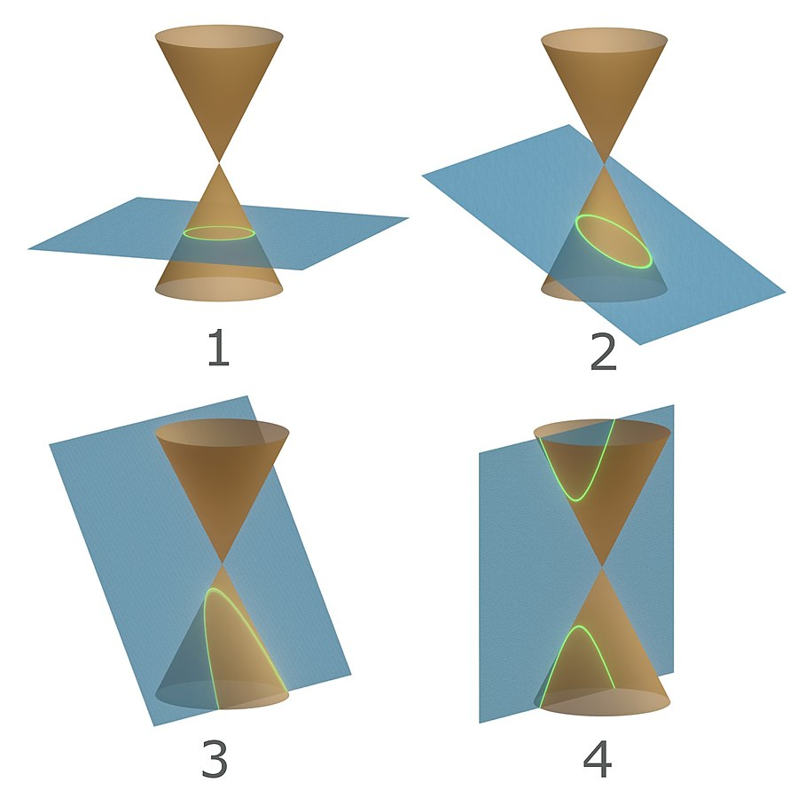
All of these conic sections are graphs of a quadratic equation of the form
$$ ax^2 + bxy + cy^2 + dx + ey + f = 0 $$
If $b=0$, then the graph of the equation can be obtained by completing the square
$$ \begin{align*} ax^2 + cy^2 + dx + ey + f &= 0 \\ a\left( x^2 + \frac{d}{a}x \right) + c\left( y^2 + \frac{e}{c}y \right) &= -f \\ a\left( x^2 + \frac{d}{a}x + \frac{d^2}{4a^2} \right) + c\left( y^2 + \frac{e}{c}y + \frac{e^2}{4c^2} \right) &= \frac{d^2}{4a} + \frac{e^2}{4c} - f \\ \\ h &:= -\frac{d}{2a} \\ k &:= -\frac{e}{2c} \\ \\ a\left(x - h\right)^2 + c\left(y - k\right)^2 &= \frac{d^2}{4a} + \frac{e^2}{4c} - f \\ \frac{(x - h)^2}{c} + \frac{(y - k)^2}{a} &= \frac{d^2}{4a^2c} + \frac{e^2}{4ac^2} - \frac{f}{ac} \\ \end{align*} $$
We usually normalize the equation by dividing both sides of the last equation by the right-hand side to obtain
- an ellipse
$$ \frac{(x-h)^2}{\alpha^2} + \frac{(y-k)^2}{\beta^2} = 1 $$
with axes of length $2\alpha$ and $2\beta$ centered at the point $(h,k)$
- a circle if the axes of the ellipse are equal, $\alpha = \beta$.
$$ (x-h)^2 + (y-k)^2 = \alpha^2 $$
- an hyperbola
$$ \frac{(x-h)^2}{\alpha^2} - \frac{(y-k)^2}{\beta^2} = \pm\,1 $$
- a parabola
$$ (x-h)^2 = 4p(y-k) $$
or
$$ (y-k)^2 = 4p(x-h) $$
The axes of these curves are parallel to the coordinate axes because there is no $\ bxy\ $ term in the general formula.
Theorem 2
The general form of the second-degree equation
$$ ax^2 + bxy + cy^2 + dx + ey + f = 0 $$ can be re-written in the form
$$ \alpha u^2 + \gamma v^2 + \delta u + \epsilon v + \zeta = 0, $$
by rotating the axis counterclockwise through the angle $\theta$, where
$$ \cot(2\theta) = \frac{a-c}{b} $$
The coefficients of the equation are obtained from the substitutions
$$ x = u\cos(\theta) - v\sin(\theta),\qquad\text{and}\qquad y = u\sin(\theta) + v\cos(\theta) $$
Proof of Theorem 2
$$ \begin{align*} ax^2 + bxy + cy^2 + dx + ey + f &= 0 \\ \\ a(u\cos(\theta) - v\sin(\theta))^2 + \quad b(u\cos(\theta) - v\sin(\theta))(u\sin(\theta) + v\cos(\theta)) + \qquad\qquad \\ \\ \qquad c(u\sin(\theta) + v\cos(\theta))^2 + d(u\cos(\theta) - v\sin(\theta)) \qquad \\ \\ \qquad\qquad e(u\sin(\theta) + v\cos(\theta)) + f &= 0 \\ \\ \\ a(u^2\cos^2(\theta) - 2uv\cos(\theta)\sin(\theta) + v^2\sin^2(\theta)) + \qquad\qquad \\ \\ \quad b(u^2\cos(\theta)\sin(\theta) + uv\cos^2(\theta) - uv\sin^2(\theta) - v^2\cos(\theta)\sin(\theta)) + \qquad\quad \\ \\ c(u^2\sin^2(\theta) + 2uv\cos(\theta)\sin(\theta) + v^2\cos^2(\theta)) + \qquad \\ \\ d(u\cos(\theta) - v\sin(\theta)) + e(u\sin(\theta) + v\cos(\theta)) + f &= 0 \\ \\ \\ a(u^2\cos^2(\theta) - uv\sin(2\theta) + v^2\sin^2(\theta)) + \qquad\qquad\quad \\ \\ b(u^2\cos(\theta)\sin(\theta) + uv\cos(2\theta) - v^2\cos(\theta)\sin(\theta)) + \qquad\qquad \\ \\ c(u^2\sin^2(\theta) + uv\sin(2\theta) + v^2\cos^2(\theta)) + d(u\cos(\theta) - v\sin(\theta)) + \qquad \\ \\ e(u\sin(\theta) + v\cos(\theta)) + f &= 0 \\ \\ \\ u^2\left(a\cos^2(\theta) + b\cos(\theta)\sin(\theta) + c\sin^2(\theta)\right) + \qquad\qquad \\ \\ uv\left(-a\sin(2\theta) + b\cos(2\theta) +c\sin(2\theta)\right) + \qquad\quad \\ \\ v^2\left(a\sin^2(\theta) - b\cos(\theta)\sin(\theta) + c\cos^2(\theta)\right) + \qquad \\ \\ u\left(d\cos(\theta) + e\sin(\theta)\right) + v\left(e\cos(\theta) - d\sin(\theta)\right) + f &= 0 \end{align*} $$
If one defines $\theta$ by
$$ \cot(2\theta) = \frac{a-c}{b} $$
then one obtains
$$ \begin{align*} b\cos(2\theta) &= (a - c)\sin(2\theta) \\ \\ 0 &= -a\sin(2\theta) + b\cos(2\theta) + c\sin(2\theta) \end{align*} $$
Substituting yields
$$\begin{align*} u^2\left(a\cos^2(\theta) + b\cos(\theta)\sin(\theta) + c\sin^2(\theta)\right) + v^2\left(a\sin^2(\theta) - b\cos(\theta)\sin(\theta) + c\cos^2(\theta)\right) + \\ \\ u\left(d\cos(\theta) + e\sin(\theta)\right) + v\left(e\cos(\theta) - d\sin(\theta)\right) + f = 0 \end{align*}$$
$$ \begin{align*} \alpha &= a\cos^2(\theta) + b\cos(\theta)\sin(\theta) + c\sin^2(\theta) \\ \beta &= 0 \\ \gamma &= a\sin^2(\theta) - b\cos(\theta)\sin(\theta) + c\cos^2(\theta) \\ \delta &= d\cos(\theta) + e\sin(\theta) \\ \epsilon &= e\cos(\theta) - d\sin(\theta) \\ \zeta &= f \end{align*} $$
This completes the proof. $\blacksquare$
Example 7
Perform a rotation of axes to eliminate the $xy$-term from
$$ 5x^2 - 6xy + 5y^2 + 14\sqrt{2}x - 2\sqrt{2}y + 18 = 0 $$
and sketch the graph in the $uv$-plane.
The angle of rotation is given by
$$ \begin{align*} \cot(2\theta) &= \frac{a - c}{b} = \frac{5 - 5}{-6} = 0 \\ \frac{\cos(2\theta)}{\sin(2\theta)} &= 0 \\ \cos(2\theta) &= 0 \\ 2\theta &= \frac{\pi}{2} + 2n\pi,\ n\in\mathbb{Z} \\ \theta &= \frac{\pi}{4} \end{align*} $$
By substituting
$$ \begin{align*} x &= u\cos(\theta) - v\sin(\theta) = \frac{u - v}{\sqrt{2}} \\ y &= u\sin(\theta) + v\cos(\theta) = \frac{u + v}{\sqrt{2}} \end{align*} $$
into the original equation one obtains
$$ 5\left(\frac{u - v}{\sqrt{2}}\right)^2 - 6\left(\frac{u - v}{\sqrt{2}}\right)\left(\frac{u + v}{\sqrt{2}}\right) + 5\left(\frac{u + v}{\sqrt{2}}\right)^2 + 14\sqrt{2}\left(\frac{u - v}{\sqrt{2}}\right) - 2\sqrt{2}\left(\frac{u + v}{\sqrt{2}}\right) + 18 = 0 $$
$$ \frac{5}{2}(u^2 - 2uv + v^2) - 3(u^2 - v^2) + \frac{5}{2}(u^2 + 2uv + v^2) + 14(u-v) - 2(u+v) + 18 = 0 $$
$$ \begin{align*} 2u^2 + 8v^2 + 12u - 16v + 18 &= 0 \\ u^2 + 4v^2 + 6u - 8v + 9 &= 0 \\ u^2 + 6u + 9 + 4\left(v^2 - 2v + 1\right) + 9 &= 9 + 4 \\ \\ (u + 3)^2 + 4(v - 1)^2 &= 4 \\ \\ \frac{(u+3)^2}{4} + \frac{(v-1)^2}{1} &= 1 \end{align*} $$
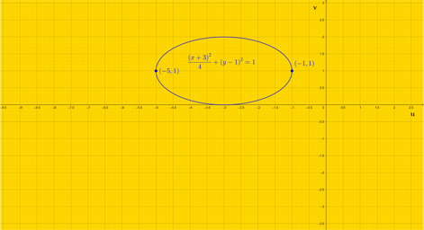
The ellipse has a semi-major axis of 2 parallel to the $u$-axis and semi-minor axis of 1 parallel to the $v$-axis. Now if we apply the transition matrix
$$ T = \begin{bmatrix} \cos\left(\frac{\pi}{4}\right) & -\sin\left(\frac{\pi}{4}\right) \\ \sin\left(\frac{\pi}{4}\right) &\ \ \cos\left(\frac{\pi}{4}\right) \end{bmatrix} = \frac{1}{\sqrt{2}}\begin{bmatrix} 1 & -1 \\ 1 &\ \ 1\end{bmatrix} $$
to every point on the ellipse in the $uv$-plane, then we have the graph of the original equation in the $xy$-plane.
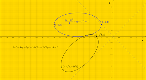
Each of the antipodal points at the ends of the semi-major axis in the $uv$-plane become
$$ \begin{align*} \begin{bmatrix} -5 \\ \ \ 1 \end{bmatrix}_{\theta} &= \frac{1}{\sqrt{2}}\begin{bmatrix} 1 & -1 \\ 1 &\ \ 1\end{bmatrix}\begin{bmatrix} -5 \\ \ \ 1 \end{bmatrix} = \begin{bmatrix} \frac{-6}{\sqrt{2}} \\ \frac{-4}{\sqrt{2}} \end{bmatrix} = \begin{bmatrix} -3\sqrt{2} \\ -2\sqrt{2} \end{bmatrix} \\ \begin{bmatrix} -1 \\ \ \ 1 \end{bmatrix}_{\theta} &= \frac{1}{\sqrt{2}}\begin{bmatrix} 1 & -1 \\ 1 &\ \ 1\end{bmatrix}\begin{bmatrix} -1 \\ \ \ 1 \end{bmatrix} = \begin{bmatrix} \frac{-2}{\sqrt{2}} \\ \frac{0}{\sqrt{2}} \end{bmatrix} = \begin{bmatrix} -\sqrt{2} \\ \ \ 0 \end{bmatrix} \end{align*} $$
in the $xy$-plane.